Dynamics of Real-Time Simulation – Chapter 5 – Dynamics of Digital-to-Analog and Analog-to-Digital Conversion
5.1 Introduction
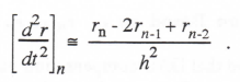
Real-time digital simulation often involves inputs and outputs in the form of analog (i.e., continuous) signals. Clearly this is true for the “hardware-in-the-loop” simulation shown in Figure 5.1, where the hardware requires continuous inputs and produces continuous outputs. In this case the continuous outputs from the hardware must be converted to digital data sequences using A to D (Analog to Digital) converters, a single channel of which is shown in the figure. The computer outputs in the form of data sequences must be converted to continuous signals using D to A (Digital to Analog) converters. Again, a single channel is shown in Figure 5.1. For both A to D and D to A converters we have assumed that the sample period h is fixed, which is almost invariably the case in real-time, hardware-in-the-loop simulation.
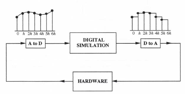
Figure 5.1. Hardware-in-the-loop flight simulation.
In this chapter we will examine the dynamics of the A to D and D to A conversion process. As in the previous chapters we will find this most convenient and meaningful in the frequency domain. In the next section we will consider D to A conversion using both zero and first-order extrapolation. The resulting DAC (Digital to Analog Converter) characteristics will be examined in the frequency domain by deriving the DAC transfer function for sinusoidal input data sequences. This will lead in subsequent sections to the development of digital algorithms to compensate for the DAC transfer function gain and phase errors. The spectral characteristics of A to D converters will be examined in the last section of this chapter.
5.2 Definition of Zero and First-order DAC extrapolation
Assume that the digital computer produces a data sequence ![]() which is converted to a continuous signal using a double-buffered DAC. The DAC data word,
which is converted to a continuous signal using a double-buffered DAC. The DAC data word, ![]() , is loaded into the outer buffer register prior to time nh, where h is the fixed time between data points. At t = nh the data word
, is loaded into the outer buffer register prior to time nh, where h is the fixed time between data points. At t = nh the data word ![]() is transferred to the inner buffer register so that the DAC output becomes the analog equivalent of
is transferred to the inner buffer register so that the DAC output becomes the analog equivalent of ![]() . Every h seconds this process is repeated, which results in the staircase function shown in Figure 5.2. The DAC output
. Every h seconds this process is repeated, which results in the staircase function shown in Figure 5.2. The DAC output ![]() in this case represents a zero-order extrapolation of the input data sequence
in this case represents a zero-order extrapolation of the input data sequence ![]() . This is the most common method of mechanizing DAC outputs in a real-time simulation.
. This is the most common method of mechanizing DAC outputs in a real-time simulation.
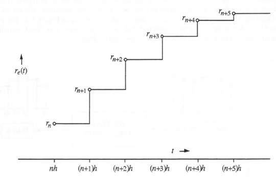
Figure 5.2. Zero-order DAC extrapolation.
An alternative is to use first-order extrapolation, which is illustrated in Figure 5.3. Here the DAC is used in combination with an analog integrator and storage device to produce a linearly-varying output over the nth sample period based on the current ![]() and previous
and previous ![]() data points.
data points.
5.3 Transfer Function for Zero-order Extrapolating DAC
We will obtain the transfer function for the DAC which uses zero-order extrapolation by taking the Fourier transform of the DAC output ![]() when the input data sequence
when the input data sequence ![]() is a sinusoid. First we define the unit data point response of the DAC, i.e., the response to the input
is a sinusoid. First we define the unit data point response of the DAC, i.e., the response to the input
(5.1) 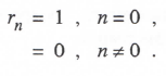
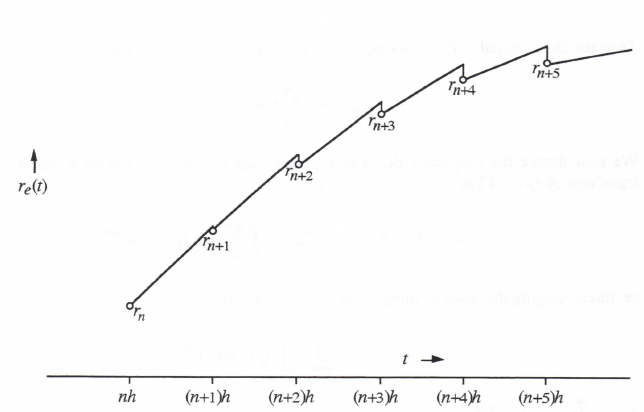
Figure 5.3. First-order DAC extrapolation.
We define the corresponding DAC response as ![]() , which is shown in Figure 5.4 in the case of zero-order extrapolation. From the figure it is apparent that
, which is shown in Figure 5.4 in the case of zero-order extrapolation. From the figure it is apparent that
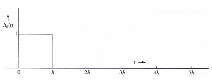
Figure 5.4. Unit data point response of zero-order DAC extrapolator.
(5.2)
Then the DAC output ![]() for any input data sequence can be represented as
for any input data sequence can be represented as
(5.3) 
We now derive the frequency domain representation of the DAC output by taking the Fourier transform of ![]() . Thus
. Thus
or, interchanging the order of integration and summation,
(5.4) 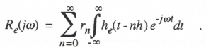
Here ![]() is the Fourier transform of
is the Fourier transform of ![]() . We recall the translation theorem of the Laplace transform, which states that
. We recall the translation theorem of the Laplace transform, which states that
![]()
The equivalent theorem for the Fourier transform states that
![]()
Thus we can rewrite Eq. (5.4) as
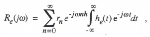
or
(5.5) 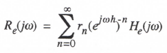
where
(5.6) 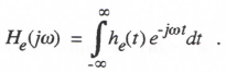
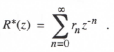
We also recall that the Z transform of the data sequence ![]() is defined as
is defined as
Hence we can write Eq. (5.5) as
(5.7) ![]()
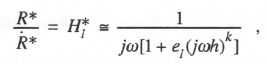
It follows that ![]() can be interpreted as representing the transfer function of the zero-order DAC extrapolator for a sinusoidal data sequence input. We can determine the formula for
can be interpreted as representing the transfer function of the zero-order DAC extrapolator for a sinusoidal data sequence input. We can determine the formula for ![]() by substituting Eq. (5.2) into (5.6). Thus
by substituting Eq. (5.2) into (5.6). Thus
(5.8) 
An alternative expression for ![]() is obtained as follows:
is obtained as follows:
(5.9) 
Figure 5.5 shows a plot of the magnitude (gain) and phase angle of ![]() versus dimensionless frequency
versus dimensionless frequency ![]() over the range
over the range ![]() . Here
. Here ![]() corresponds to
corresponds to ![]() , the data sequence sample frequency in radians per second. In Figure 5.5 the gain is normalized by plotting
, the data sequence sample frequency in radians per second. In Figure 5.5 the gain is normalized by plotting ![]() , which from Eq. (5.9) is given by
, which from Eq. (5.9) is given by ![]() . The phase angle is given by
. The phase angle is given by ![]() . The resulting linear phase lag with frequency is apparent in Figure 5.5. This phase characteristic corresponds to a pure time delay of h/2 seconds, which is also intuitively obvious in Figure 5.2 when a smoothed curve through the staircase function is compared with the data sequence driving the DAC.
. The resulting linear phase lag with frequency is apparent in Figure 5.5. This phase characteristic corresponds to a pure time delay of h/2 seconds, which is also intuitively obvious in Figure 5.2 when a smoothed curve through the staircase function is compared with the data sequence driving the DAC.
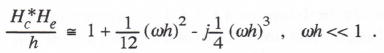
If we make a power series expansion of the zero-order extrapolator transfer function in Eq. (5.8), the following formula is obtained:
(5.10) 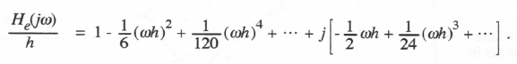
Ideally, the DAC extrapolator transfer function, ![]() , should be 1, i.e., the DAC output for a sinusoidal input should be a sinusoid of the same amplitude with no phase shift. From Eq. (5.10) it is easy to show that the DAC gain error,
, should be 1, i.e., the DAC output for a sinusoidal input should be a sinusoid of the same amplitude with no phase shift. From Eq. (5.10) it is easy to show that the DAC gain error, ![]() , and the phase error,
, and the phase error, ![]() , are given by the following approximate formulas
, are given by the following approximate formulas
(5.11) 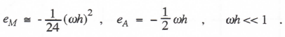
Note in this case that the approximate gain error is not equal to the real part, ![]() , of the fractional error in DAC transfer function, as stated earlier in Eq. (1.53). This is because here the real part of the fractional transfer function error is of order
, of the fractional error in DAC transfer function, as stated earlier in Eq. (1.53). This is because here the real part of the fractional transfer function error is of order ![]() , whereas the imaginary part of the fractional transfer function error is of order h. Thus the imaginary part as well as the real part make contributions of order
, whereas the imaginary part of the fractional transfer function error is of order h. Thus the imaginary part as well as the real part make contributions of order ![]() to the gain error.
to the gain error.
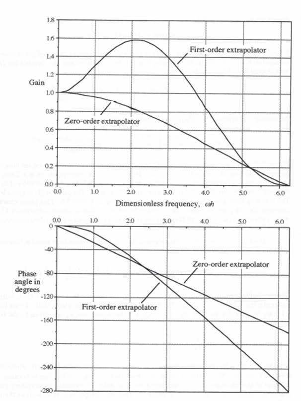
Figure 5.5. Frequency Response of zero and first-order DAC extrapolators
5.4. Transfer Function for First-order Extrapolating DAC
The unit data point response for the first-order DAC extrapolator illustrated in Figure 5.3 is shown in Figure 5.6. It is given by the formula
(5.13) 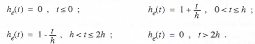
When we take the Fourier transform of Eq. (5.13) using Eq. (5.6), the following formula is obtained for the first-order extrapolator transfer function:
(5.14) 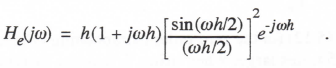
Plots of the normalized gain, ![]() , and the phase angle of
, and the phase angle of ![]() are shown as a function of dimensionless frequency
are shown as a function of dimensionless frequency ![]() in Figure 5.5. Note that the gain exhibits a peak of approximately 1.6 at about one-third the sample frequency. By comparison, the transfer function gain for the zero-order extrapolator has no peaking. Also, at low frequencies the phase lag for the first-order extrapolator is quite small compared to the phase lag for the zero-order extrapolator. However, at higher frequencies the first-order extrapolator exhibits a larger lag.
in Figure 5.5. Note that the gain exhibits a peak of approximately 1.6 at about one-third the sample frequency. By comparison, the transfer function gain for the zero-order extrapolator has no peaking. Also, at low frequencies the phase lag for the first-order extrapolator is quite small compared to the phase lag for the zero-order extrapolator. However, at higher frequencies the first-order extrapolator exhibits a larger lag.
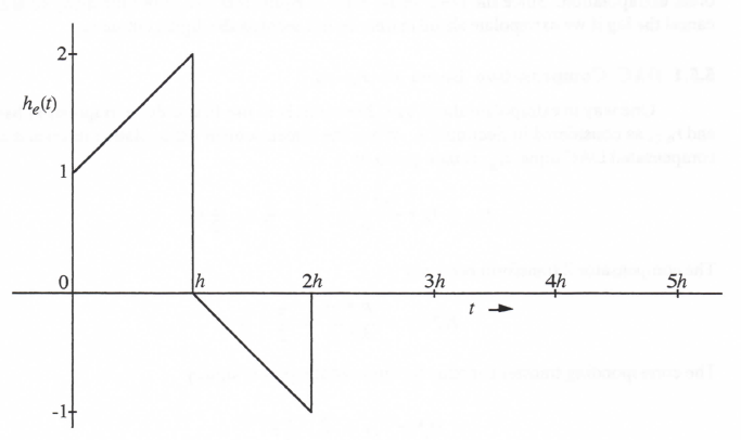
Figure 5.6. Unit data point response for first-order DAC extrapolator.
When we make a power series expansion of the first-order extrapolator transfer function in Eq. (5.14), the following formula is obtained:
(5.15) 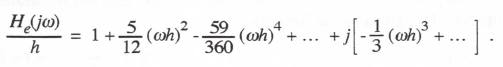
Here the real and imaginary parts of ![]() represent, respectively, the approximate fractional gain error,
represent, respectively, the approximate fractional gain error, ![]() , and the phase error,
, and the phase error, ![]() , of the first-order extrapolator. This is in accordance with Eqs. (1.53) and (1.54), which apply in this case since the order of the phase error is higher than half the order of the gain error. Thus we can write
, of the first-order extrapolator. This is in accordance with Eqs. (1.53) and (1.54), which apply in this case since the order of the phase error is higher than half the order of the gain error. Thus we can write
(5.16) 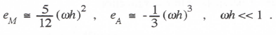
Comparison with Eq. (5.12) for the zero-order extrapolating DAC shows that for ![]() the gain error magnitude is 2.5 times larger when using first-order extrapolation. For both schemes the gain varies as
the gain error magnitude is 2.5 times larger when using first-order extrapolation. For both schemes the gain varies as ![]() . Again, comparison of Eqs. (5.12) and (5.16) shows that for
. Again, comparison of Eqs. (5.12) and (5.16) shows that for ![]() the phase error is much larger in the case of the zero-order extrapolating DAC. Specifically, in the zero-order DAC the phase error is proportional to the first power of the sample period h and will be the predominant cause of dynamic errors when using zero-order extrapolating DAC’s.
the phase error is much larger in the case of the zero-order extrapolating DAC. Specifically, in the zero-order DAC the phase error is proportional to the first power of the sample period h and will be the predominant cause of dynamic errors when using zero-order extrapolating DAC’s.
5.5 Digital Compensation of Zero-order Extrapolating DAC’s.
In this section we consider means for compensating the dynamic errors produced by zero-order extrapolation. Since the DAC phase error is equivalent to a pure time delay of ![]() , we can cancel the lag if we extrapolate ahead in time by
, we can cancel the lag if we extrapolate ahead in time by ![]() seconds the digital output
seconds the digital output ![]() .
.
5.5.1 DAC Compensation Based on ![]()
One way to extrapolate ahead by ![]() seconds is to use first-order extrapolation based on
seconds is to use first-order extrapolation based on ![]() , and
, and ![]() , as considered in Section 4.1. When the dimensionless extrapolation interval
, as considered in Section 4.1. When the dimensionless extrapolation interval ![]() , the compensated DAC input,
, the compensated DAC input, ![]() , is then given by
, is then given by
(5.17) 
The compensator Z transform becomes
(5.18) 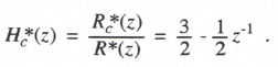
The corresponding transfer function for sinusoidal inputs is simply
(5.19) 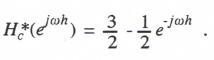
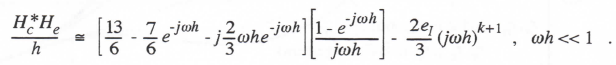
The product of the compensator transfer function and the normalized DAC transfer function, ![]() , as obtained from Eq. (5.8), becomes
, as obtained from Eq. (5.8), becomes
(5.20) 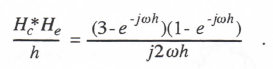
Expanding ![]() in a power series and retaining terms up to order
in a power series and retaining terms up to order ![]() , we obtain the following approximate formula for the combined transfer function:
, we obtain the following approximate formula for the combined transfer function:
(5.21) 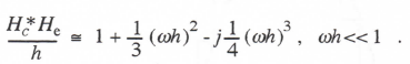
Ideally, ![]() should equal 1 if the DAC compensation is complete. As before, we note that the terms
should equal 1 if the DAC compensation is complete. As before, we note that the terms ![]() and
and ![]() on the right side of Eq. (5.21) represent, respectively, the approximate gain and phase errors in
on the right side of Eq. (5.21) represent, respectively, the approximate gain and phase errors in ![]() . Figure 5.7 shows the DAC response to a sinusoidal data sequence without and with compensation based on
. Figure 5.7 shows the DAC response to a sinusoidal data sequence without and with compensation based on ![]() and
and ![]() .. The effectiveness of the compensation in removing the half-step lag in DAC output is clearly evident.
.. The effectiveness of the compensation in removing the half-step lag in DAC output is clearly evident.
5.5.2 DAC Compensation Based on ![]()
Next we let the compensation of the half-frame lag associated with the zero-order extrapolator be based on extrapolation using ![]() and
and ![]() . This requires, of course, that
. This requires, of course, that ![]() is a state variable or is explicitly related to state variables so that
is a state variable or is explicitly related to state variables so that ![]() can be calculated. In this case the formula for the compensated output becomes
can be calculated. In this case the formula for the compensated output becomes
(5.22) ![]()
And the compensator transfer function for sinusoidal inputs is simply
(5.23) 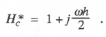
The product of the compensator transfer function and the normalized DAC transfer function now becomes
(5.24) 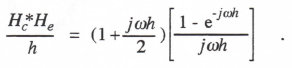
Expanding ![]() in a power series, we obtain the following approximate formula for the combined transfer function:
in a power series, we obtain the following approximate formula for the combined transfer function:
(5.25) 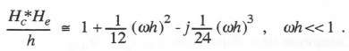
Again the compensator has cancelled the first-order phase error in the DAC transfer function. However, comparison of Eq. (5.25) with (5.21) shows that the compensator based on ![]() and
and ![]() produces residual gain and phase errors which are only 1/4 and 1/6 times as much, respectively, as the corresponding errors when the compensation is based on
produces residual gain and phase errors which are only 1/4 and 1/6 times as much, respectively, as the corresponding errors when the compensation is based on ![]() and
and ![]() . Clearly the compensation based on
. Clearly the compensation based on ![]() and
and ![]() , is preferable. Eqs. (5.21) and (5.25) are of course valid only for
, is preferable. Eqs. (5.21) and (5.25) are of course valid only for ![]() .
.
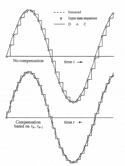
Figure 5.7. DAC response to sinusoidal input without and with compensation
based on ![]()
5.5.3 DAC Compensation Based on ![]()
In both Eqs. (5.21) and (5.25) it is apparent that the dominant error in the combined compensator-DAC transfer function is proportional to ![]() . This suggests that an incremental compensation proportional to
. This suggests that an incremental compensation proportional to ![]() can be used to cancel these errors. To find such a compensation we note that the sinusoidal function,
can be used to cancel these errors. To find such a compensation we note that the sinusoidal function, ![]() , has a second derivative,
, has a second derivative, ![]() , which is given by
, which is given by ![]() . The following formula represents a numerical approximation to the second derivative:
. The following formula represents a numerical approximation to the second derivative:
This in turn suggests that we consider a compensation increment proportional to
(5.26) ![]()
Taking the Z transform of Eq. (5.26) and solving for the incremental transfer function ![]() , we obtain
, we obtain
![]()
The incremental transfer function for sinusoidal inputs is then given by
(5.27) ![]()
Expanding the exponential functions in power series, we have
(5.28) 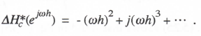
From Eq. (5.21) we see that the desired incremental transfer function is equal to ![]() , i.e.,
, i.e., ![]() based on Eq. (5.28). Thus we add
based on Eq. (5.28). Thus we add ![]() , or from Eq. (5.26),
, or from Eq. (5.26), ![]() , to the original compensator equation (5.17). This results in the new compensator equation
, to the original compensator equation (5.17). This results in the new compensator equation
(5.29) 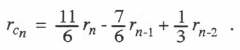
After taking the Z transform, replacing z by ![]() , and solving for the compensator transfer function, we obtain
, and solving for the compensator transfer function, we obtain
(5.31) 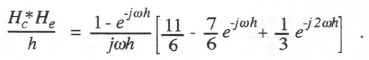
From Eq. (5.8) the combined compensator-DAC transfer function now becomes
(5.31) 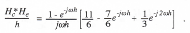
Expanding the exponential functions in power series and retaining terms up to h4, we obtain
(5.32) 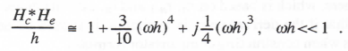
Eq. (5.32) shows that the DAC compensator algorithm of Eq. (5.29) has eliminated the gain error of ![]() in the earlier combined compensator-DAC transfer function in Eq. (2.8). The Predominant error for
in the earlier combined compensator-DAC transfer function in Eq. (2.8). The Predominant error for ![]() is now the phase error,
is now the phase error, ![]() .
.
5.5.4 DAC Compensation Based on ![]()
In Section 5.5.2 we found that DAC compensation using ![]() and
and ![]() gave better results than the compensation using
gave better results than the compensation using ![]() and
and ![]() in Section 5.5.1. If
in Section 5.5.1. If ![]() is available, then the following formula can be used to define an incremental compensation
is available, then the following formula can be used to define an incremental compensation ![]() proportional to
proportional to ![]() , as needed to cancel transfer function errors proportional to
, as needed to cancel transfer function errors proportional to ![]() :
:
(5.33) ![]()
This formula is based on ![]() representing a central difference approximation to
representing a central difference approximation to ![]() . It follows that
. It follows that ![]() represents an approximation to
represents an approximation to ![]() , which leads directly to Eq. (5.33). The incremental compensator transfer function is given by
, which leads directly to Eq. (5.33). The incremental compensator transfer function is given by
(5.34) ![]()
Expanding the exponential function in a power series, we obtain
(5.35) ![]()
Comparison with Eq. (5.25) shows that ![]() in Eq. (5.35) must be multiplied by 1/6 to produce the increment
in Eq. (5.35) must be multiplied by 1/6 to produce the increment ![]() which, when added to Eq. (5.25), will cancel the error of order
which, when added to Eq. (5.25), will cancel the error of order ![]() . Thus the new compensator algorithm is obtained by adding 1/6 times the
. Thus the new compensator algorithm is obtained by adding 1/6 times the ![]() of Eq. (5.33) to the right side of Eq. (5.22) to produce the following compensator formula:
of Eq. (5.33) to the right side of Eq. (5.22) to produce the following compensator formula:
(5.36) 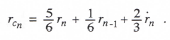
Following the same procedure used earlier to derive the combined compensator-DAC transfer function in Eq. (5.31), we obtain
(5.37) 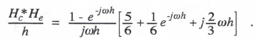
Expanding the exponential functions in power series and retaining terms up to ![]() , we have
, we have
(5.38) 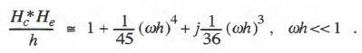
Comparison with Eq. (5.32) for compensation based on ![]() , and
, and ![]() shows that the compensation here, which is based on
shows that the compensation here, which is based on ![]() and
and ![]() , exhibits much smaller gain and phase errors. Again, we see that if the derivative
, exhibits much smaller gain and phase errors. Again, we see that if the derivative ![]() is available, it should be used in preference to past data sequence values when constructing compensator formulas.
is available, it should be used in preference to past data sequence values when constructing compensator formulas.
5.5.4 DAC Compensation Based on ![]()
In Section 4.6 we considered extrapolation based on ![]() and
and ![]() as an alternative to extrapolation based on
as an alternative to extrapolation based on ![]() and
and ![]() . This may be necessary when r is a state variable but
. This may be necessary when r is a state variable but ![]() is not, in which case
is not, in which case ![]() is not calculated in the nth frame. Then the following formula based on
is not calculated in the nth frame. Then the following formula based on ![]() and
and ![]() can be used to define an incremental compensation
can be used to define an incremental compensation ![]() proportional to
proportional to ![]() , as needed to cancel transfer function errors proportional to
, as needed to cancel transfer function errors proportional to ![]() :
:
(5.39) ![]()
As before, this formula is based on ![]() representing a central difference approximation to
representing a central difference approximation to ![]() . It follows that
. It follows that ![]() represents an approximation to
represents an approximation to ![]() , which leads directly to Eq. (5.39). The incremental compensator transfer function is now given by
, which leads directly to Eq. (5.39). The incremental compensator transfer function is now given by
(5.40) ![]()
Expanding the exponential function in a power series, we obtain
(5.41) 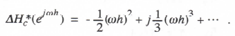
Comparison with Eq. (5.21) shows that ![]() in Eq. (5.35) must be multiplied by 2/3 to produce the increment
in Eq. (5.35) must be multiplied by 2/3 to produce the increment ![]() which, when added to Eq. (5.21), will cancel the error of order
which, when added to Eq. (5.21), will cancel the error of order ![]() . Thus the new compensator algorithm is obtained by adding 2/3 times the
. Thus the new compensator algorithm is obtained by adding 2/3 times the ![]() of Eq. (5.39) to the right side of Eq. (5.17) to produce the following compensator formula:
of Eq. (5.39) to the right side of Eq. (5.17) to produce the following compensator formula:
(5.42) 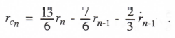
The combined compensator-DAC transfer function is then given by
(5.43) 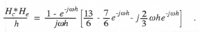
Expanding the exponential functions in power series and retaining terms up to ![]() , we have
, we have
(5.44) 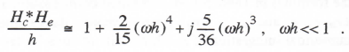
.
Comparison with Eq. (532) for compensation based on ![]() and
and ![]() shows that the compensation here, which is based on
shows that the compensation here, which is based on ![]() and
and ![]() , exhibits smaller gain and phase errors. On the other hand the errors are larger than those in Eq. (5.38) for compensation based on
, exhibits smaller gain and phase errors. On the other hand the errors are larger than those in Eq. (5.38) for compensation based on ![]() and
and ![]() .
.
5.6. Summary of Methods for Dynamic Compensation of D to A Convertors
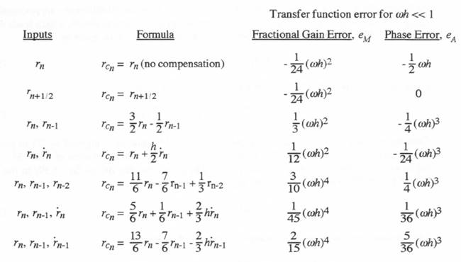
Table 5.1 summarizes the different methods considered for DAC compensation in this chapter. Listed for each method are the required inputs, the compensator formula, and the approximate fractional gain error, ![]() , and phase error,
, and phase error, ![]() , for the combined compensator-DAC transfer function. Also listed in the table are the gain and phase errors for the uncompensated DAC. As noted earlier, the approximate gain and phase errors are equal to the real and imaginary parts, respectively, of the fractional error in transfer function. The one exception to this, as noted in Section 53, is in the case of the uncompensated DAC transfer function, where the gain error is not simply the real part of the fractional error in transfer function.
, for the combined compensator-DAC transfer function. Also listed in the table are the gain and phase errors for the uncompensated DAC. As noted earlier, the approximate gain and phase errors are equal to the real and imaginary parts, respectively, of the fractional error in transfer function. The one exception to this, as noted in Section 53, is in the case of the uncompensated DAC transfer function, where the gain error is not simply the real part of the fractional error in transfer function.
Table 5.1
Summary of Compensator Formulas and Combined Compensator-DAC Transfer
Function Errors for Sinusoidal Input Data Sequences
5.7 Effect of Integration Errors for Compensation Formulas Using ![]()
In deriving the formulas in Table 5.1 for combined compensator-DAC transfer function errors, we assumed that ![]() and
and ![]() for a sinusoidal data sequence
for a sinusoidal data sequence ![]() . In fact, when r is determined by numerical integration of
. In fact, when r is determined by numerical integration of ![]() , which will always be true in a digital simulation for which r is a state variable,
, which will always be true in a digital simulation for which r is a state variable, ![]() is actually related to
is actually related to ![]() by the transfer function
by the transfer function ![]() of the numerical integrator. In Chapter 3 we derived both exact and approximate formulas for
of the numerical integrator. In Chapter 3 we derived both exact and approximate formulas for ![]() for a number of numerical methods. In particular, we determined in Eq. (3.37) the following general form for the integrator transfer function:
for a number of numerical methods. In particular, we determined in Eq. (3.37) the following general form for the integrator transfer function:
or
(5.45)
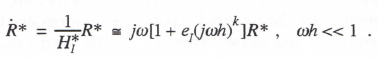
It follows that
(5.46) 
5-14
Thus ![]() should be replaced by
should be replaced by ![]() , not simply
, not simply ![]() , in deriving formulas for the DAC-compensator transfer function
, in deriving formulas for the DAC-compensator transfer function ![]() , where
, where ![]() can be expressed in either the exact or approximate form for any given integration algorithm. For example, Eq. (5.23) for the compensator transfer function based on
can be expressed in either the exact or approximate form for any given integration algorithm. For example, Eq. (5.23) for the compensator transfer function based on ![]() , and
, and ![]() is then replaced by
is then replaced by
(5.47) 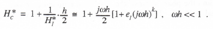
Then the combined compensator-DAC transfer function, ![]() becomes
becomes
(5.48) 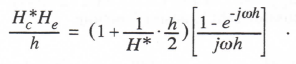
Eq. (5.48) is exact. When the approximate representation of ![]() is used, the formula becomes
is used, the formula becomes
(5.49) 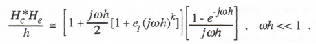
If the order k of the integration algorithm is equal to or greater than the order of the compensator algorithm, which here is 2, then the approximate formula for the combined compensator-DAC transfer function can be written as
(5.50) 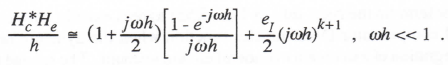
The first term on the right side of Eq. (5.50) agrees exactly with Eq. (5.24) and represents the combined compensator-DAC transfer function when the dynamic error associated with the numerical integration of ![]() to obtain r is not taken into account. The second term on the right side of Eq. (5.50) represents the contribution of the integrator error to the overall compensator-DAC transfer function error. To illustrate, consider the case where the AB-2 algorithm is used to integrate
to obtain r is not taken into account. The second term on the right side of Eq. (5.50) represents the contribution of the integrator error to the overall compensator-DAC transfer function error. To illustrate, consider the case where the AB-2 algorithm is used to integrate ![]() to obtain r. Substituting Eq. (3.35) for the AB-2 integrator transfer function into Eq. (5.48), we obtain the following formula for the exact transfer function of the combined compensator-DAC:
to obtain r. Substituting Eq. (3.35) for the AB-2 integrator transfer function into Eq. (5.48), we obtain the following formula for the exact transfer function of the combined compensator-DAC:
(5.51) 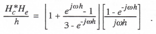
Noting that ![]() and
and ![]() for AB-2 integration and using Eq. (5.25) to represent the first term on the right side of Eq. (5.50), we obtain the following approximate formula for the combined compensator-DAC transfer function:
for AB-2 integration and using Eq. (5.25) to represent the first term on the right side of Eq. (5.50), we obtain the following approximate formula for the combined compensator-DAC transfer function:
(5.52) 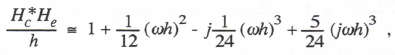
or
(5.53)
Comparison with Eq. (5.25) shows that the dominant gain error, ![]() , has not been changed as a result of including the dynamics of the AB-2 integrator in the analysis, but the phase error of order
, has not been changed as a result of including the dynamics of the AB-2 integrator in the analysis, but the phase error of order ![]() has changed from
has changed from ![]() to
to ![]() . If we had used the RTAM-2 algorithm instead of AB-2 in integrating
. If we had used the RTAM-2 algorithm instead of AB-2 in integrating ![]() to obtain r, where from Table 3.1 on page 85 we see that
to obtain r, where from Table 3.1 on page 85 we see that ![]() and
and ![]() , then the phase error of the combined compensator-DAC transfer function is approximately equal to
, then the phase error of the combined compensator-DAC transfer function is approximately equal to ![]() or
or ![]() . The approximate gain error remains equal to
. The approximate gain error remains equal to ![]() .
.
As another example, consider DAC compensation based on ![]() and
and ![]() , as described in Section 5.5.4. Replacing
, as described in Section 5.5.4. Replacing ![]() in Eq. (5.37) with
in Eq. (5.37) with ![]() , we obtain the following formula for the combined compensator-DAC transfer function:
, we obtain the following formula for the combined compensator-DAC transfer function:
(5.54) 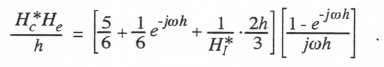
If the order k of the integration algorithm is equal to or greater than the order of the compensator algorithm, which here is 3, then the approximate formula for the combined compensator-DAC transfer function can be written as
(5.55) 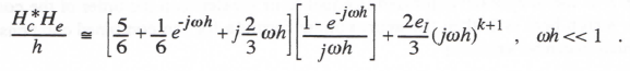
Again, the first term on the right side of Eq. (5.55) agrees exactly with Eq. (5.37) and represents the combined compensator-DAC transfer function when the dynamic error associated with the numerical integration of ![]() to obtain
to obtain ![]() is not taken into account. The second term on the right side of Eq. (5.55) represents the contribution of the integrator dynamic error to the overall compensator-DAC transfer function error. To illustrate, consider the case where the AB-3 algorithm is used in integrating
is not taken into account. The second term on the right side of Eq. (5.55) represents the contribution of the integrator dynamic error to the overall compensator-DAC transfer function error. To illustrate, consider the case where the AB-3 algorithm is used in integrating ![]() to obtain
to obtain ![]() . From Eq. (3.71) it is apparent that the AB-3 integrator transfer function for sinusoidal inputs is given by
. From Eq. (3.71) it is apparent that the AB-3 integrator transfer function for sinusoidal inputs is given by ![]() . Substitution into Eq. (5.55) leads in this case to the following formula for the exact transfer function of the combined compensator-DAC when the compensation is based on
. Substitution into Eq. (5.55) leads in this case to the following formula for the exact transfer function of the combined compensator-DAC when the compensation is based on ![]() and
and ![]() and the integration of
and the integration of ![]() to obtain r is accomplished with AB-3 integration:
to obtain r is accomplished with AB-3 integration:
(5.56) 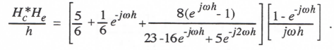
Noting that ![]() and k =3 for AB-3 integration and using Eq. (538) to represent the first term on the right side of Eq. (5.50), we obtain the following approximate formula for the combined compensator-DAC transfer function:
and k =3 for AB-3 integration and using Eq. (538) to represent the first term on the right side of Eq. (5.50), we obtain the following approximate formula for the combined compensator-DAC transfer function:
(5.57) 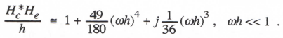
Comparison with Eq. (5.38) shows that the dominant phase error, ![]() , has not been changed as a result of including the dynamics of the AB-3 integrator in the analysis, but the phase error of order
, has not been changed as a result of including the dynamics of the AB-3 integrator in the analysis, but the phase error of order ![]() has changed from
has changed from ![]() to
to ![]() a substantial increase. The calculation of the approximate gain error for DAC-compensation based on
a substantial increase. The calculation of the approximate gain error for DAC-compensation based on ![]() and
and ![]() , when using an algorithm other than AB-3 for integrating
, when using an algorithm other than AB-3 for integrating ![]() to obtain r only requires substitution of the appropriate values for
to obtain r only requires substitution of the appropriate values for ![]() and k into Eq. (5.55).
and k into Eq. (5.55).
As a final example we consider DAC compensation based on ![]() and
and ![]() , as described in Section 5.5.4. Replacing
, as described in Section 5.5.4. Replacing ![]() in Eq. (5.43) with
in Eq. (5.43) with ![]() , we obtain the following formula for the transfer function of the combined compensator:
, we obtain the following formula for the transfer function of the combined compensator:
(5.58) 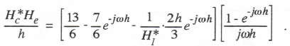
Once again, if the order k of the integration algorithm is equal to or greater than the order of the third-order compensator algorithm used here, then the approximate formula for the combined compensator-DAC transfer function can be written as
(5.59)
For the case where the AB-3 algorithm is used in integrating ![]() to obtain r the following formula for the exact transfer function of the combined compensator-DAC when the compensation is based on
to obtain r the following formula for the exact transfer function of the combined compensator-DAC when the compensation is based on ![]() and
and ![]() is obtained
is obtained
(5.60) 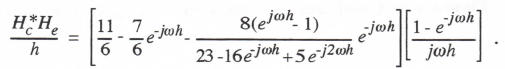
Following the same procedure used above to derive Eq. (5.56), we obtain the following formula for the approximate compensator-DAC transfer function:
(5.61) 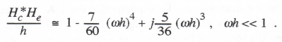
Comparison with Eq. (5.44) shows that the dominant phase error, proportional to ![]() , is unchanged by including the AB-3 integrator dynamics, but the gain error, proportional to
, is unchanged by including the AB-3 integrator dynamics, but the gain error, proportional to ![]() , is different, which is as expected.
, is different, which is as expected.
5.8 Compensator-DAC Gain Errors for ![]()
The asymptotic formulas for transfer function gain and phase errors, as derived above for the various compensator algorithms, are, of course, only valid for ![]() , where
, where ![]() is the frequency and h is the step size. In each case we also derived exact transfer function formulas, i.e., those given in Eqs. (5.9), (5.20), (5.31), (5.50), (5.56) and (5.60). From the magnitude of the complex number represented by each transfer function we can calculate the exact transfer function gain. For all five schemes, as well as the uncompensated case, plots of the exact
is the frequency and h is the step size. In each case we also derived exact transfer function formulas, i.e., those given in Eqs. (5.9), (5.20), (5.31), (5.50), (5.56) and (5.60). From the magnitude of the complex number represented by each transfer function we can calculate the exact transfer function gain. For all five schemes, as well as the uncompensated case, plots of the exact ![]() versus
versus ![]() are shown in Figure 5.8 for
are shown in Figure 5.8 for ![]() up to
up to ![]() , which corresponds to the sample frequency of the data sequence. Note the substantial peaking at about one-half the sample frequency when the compensation is based on either
, which corresponds to the sample frequency of the data sequence. Note the substantial peaking at about one-half the sample frequency when the compensation is based on either ![]() and
and ![]() , or
, or ![]() and
and ![]() . This could conceivably cause difficulties in a hardware-in-the-loop simulation in the unlikely case that the digital computer output driving the DAC contains significant components in this frequency regime.
. This could conceivably cause difficulties in a hardware-in-the-loop simulation in the unlikely case that the digital computer output driving the DAC contains significant components in this frequency regime.
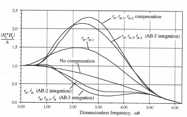
Figure 5.8. Combined compensator-DAC gain versus frequency.
5.9 Use of Multi-rate DAC Outputs to Improve Dynamic Performance
Up to this point all of our discussion of D to A converters has assumed that the DAC’s themselves are zero-order extrapolators. This means that the DAC output remains at its present value until updated to a new value with the next digital data-sequence input. This is clearly evident in Figure 5.7. It is possible to add additional analog circuitry to each DAC to convert it to a first-order extrapolator. This means that the DAC produces an analog output which is a linear extrapolation based on the current and past data sequence input values. As we have seen in Section 5.4, this has the potential of significantly reducing dynamic errors associated with the D to A conversion process, especially for ![]() . However, first-order extrapolation is accomplished at the expense of added analog complexity and is generally not used in practice. In this section we show how comparable or better improvement in performance can be achieved using multi-rate inputs to zero-order extrapolating DAC’s. The multi-rate inputs are generated using the digital extrapolation algorithms described and analyzed in Chapter 4.
. However, first-order extrapolation is accomplished at the expense of added analog complexity and is generally not used in practice. In this section we show how comparable or better improvement in performance can be achieved using multi-rate inputs to zero-order extrapolating DAC’s. The multi-rate inputs are generated using the digital extrapolation algorithms described and analyzed in Chapter 4.
For example, consider the generation of a multi-rate DAC input using extrapolation based on ![]() and
and ![]() . As in Section 4.2, we define the extrapolation time interval as
. As in Section 4.2, we define the extrapolation time interval as ![]() , where a is a dimensionless constant and h is the time-step size. From Eq. (4.2) the extrapolation formula is given by
, where a is a dimensionless constant and h is the time-step size. From Eq. (4.2) the extrapolation formula is given by
(5.62) 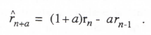
Using Eq. (5.62), we will now define an equally-spaced sequence of N data-points over the interval ![]() in order to drive a multi-rate DAC. The N DAC inputs over the nth frame will occur at
in order to drive a multi-rate DAC. The N DAC inputs over the nth frame will occur at ![]() . In order to compensate for the half-step delay inherent in the zero-order DAC, the data sequence values driving the DAC over the nth frame are advanced in time by one-half of the fast frame period, i.e.,
. In order to compensate for the half-step delay inherent in the zero-order DAC, the data sequence values driving the DAC over the nth frame are advanced in time by one-half of the fast frame period, i.e., ![]() . This means that the N DAC inputs are actually provided at
. This means that the N DAC inputs are actually provided at ![]() , respectively. For N = 4 (4 DAC updates per slow frame) Figure 5.9 shows the resulting DAC output for a portion of an input sinusoidal cycle with
, respectively. For N = 4 (4 DAC updates per slow frame) Figure 5.9 shows the resulting DAC output for a portion of an input sinusoidal cycle with ![]() = 0.25. Figure 5.10 shows the result for N = 10. As N becomes large, it is clear that the multi-rate DAC output will approach the continuous (i.e., analog) output associated with a DAC that uses first-order rather than zero-order extrapolation.
= 0.25. Figure 5.10 shows the result for N = 10. As N becomes large, it is clear that the multi-rate DAC output will approach the continuous (i.e., analog) output associated with a DAC that uses first-order rather than zero-order extrapolation.
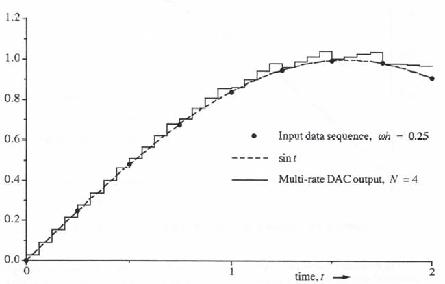
Figure 5.9. Multi-rate DAC output for N = 4 based on ![]()
The accuracy of the fast data sequence used to drive the DAC’s can be further improved by using formulas based on quadratic rather than linear extrapolation. For example, we can base the extrapolation on ![]() , and
, and ![]() . In this case the quadratic curve passes through the data points
. In this case the quadratic curve passes through the data points ![]() and
and ![]() , and matches the slope
, and matches the slope ![]() at
at ![]() . We have seen in Eq. (4.28) that the extrapolation formula is then given by
. We have seen in Eq. (4.28) that the extrapolation formula is then given by
(5.63) ![]()
Figure 5.11 shows the resulting multi-rate DAC output with N = 10 when the slow data sequence again is a portion of a sinusoidal cycle with ![]() = 0.25. Comparison with Figures 5.9 and 5.10 demonstrates the additional accuracy obtained by using quadratic instead of linear extrapolation to obtain the multi-rate DAC output.
= 0.25. Comparison with Figures 5.9 and 5.10 demonstrates the additional accuracy obtained by using quadratic instead of linear extrapolation to obtain the multi-rate DAC output.
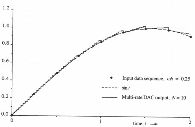
Figure 5.10. Multi-rate DAC output for N = 10 based on ![]() ,
,
The dynamic error of the DAC output in Figure 5.11 can be estimated by adding the error associated with the multi-rate data sequence to the error associated with the zero-order DAC. From Table 43 we see that the dominant error in the multi-rate data sequence when using extrapolation based on ![]() , and
, and ![]() is the phase error
is the phase error ![]() , which is equal to 0.0972
, which is equal to 0.0972 ![]() for an input sinusoid of frequency
for an input sinusoid of frequency ![]() , sample-period h, and a frame multiple of
, sample-period h, and a frame multiple of ![]() . For N = 10 the result will be very nearly the same as for
. For N = 10 the result will be very nearly the same as for ![]() . With
. With ![]() = 0.25, as in Figure 5.11, it follows that the phase error
= 0.25, as in Figure 5.11, it follows that the phase error ![]() radians. From Table 4.3 the fractional gain error is given by
radians. From Table 4.3 the fractional gain error is given by ![]() . To these errors in the fundamental component of the multi-rate data sequence used to drive the DAC we must add the dynamic error of the zero-order DAC. Because the half-frame delay associated with the DAC has been exactly compensated by advancing in time the multi-rate DAC input by 0.5h/N seconds, there will be no phase error associated with the DAC itself. Since the sample period associated with the DAC is h/N, we see from Eq. (5.11) that the DAC gain error
. To these errors in the fundamental component of the multi-rate data sequence used to drive the DAC we must add the dynamic error of the zero-order DAC. Because the half-frame delay associated with the DAC has been exactly compensated by advancing in time the multi-rate DAC input by 0.5h/N seconds, there will be no phase error associated with the DAC itself. Since the sample period associated with the DAC is h/N, we see from Eq. (5.11) that the DAC gain error ![]() . Thus the total gain error in the DAC output in Figure 5.11 is given approximately by
. Thus the total gain error in the DAC output in Figure 5.11 is given approximately by ![]() , whereas the phase error is approximately equal to 0.0015 radians. If the DAC had been driven directly by the sinusoidal data sequence with
, whereas the phase error is approximately equal to 0.0015 radians. If the DAC had been driven directly by the sinusoidal data sequence with ![]() = 0.25 instead of the multi-rate data sequence (N = 10) with a half-frame lead, we see from Eq. (5.11) that the gain error would be
= 0.25 instead of the multi-rate data sequence (N = 10) with a half-frame lead, we see from Eq. (5.11) that the gain error would be ![]() and the phase error would be – (0.25)/2 = – 0.125 radians. The accuracy improvement obtained by using the multi-rate DAC output with a half-frame advance is very apparent, especially in the phase error.
and the phase error would be – (0.25)/2 = – 0.125 radians. The accuracy improvement obtained by using the multi-rate DAC output with a half-frame advance is very apparent, especially in the phase error.
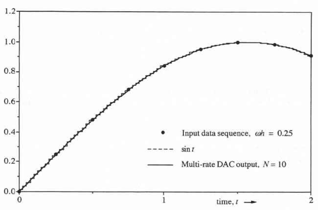
Figure 5.11. Multi-rate DAC output for N = 10 based on ![]()
5.10 Dynamics of Analog-to-digital Conversion
When a real-time digital simulation requires inputs from physical systems with continuous (analog) outputs, then conversion of the continuous signals to digital data sequences is required. This is accomplished for each continuous input by means of an ADC (analog-to-digital converter). Each ADC requires a finite conversion time, usually short compared with the interval h between samples. Sometimes a single ADC is used for a number of analog input channels, in which case a multiplexer switch much be used to connect the ADC to successive input channels. Under these circumstances it is necessary to buffer each analog channel with a sample-hold circuit if time skew is to be avoided. Then all of the analog channels can be sampled simultaneously and held at their sampled value while the multiplexed ADC successively converts each signal to digital form.
With the advent of low-cost, monolithic ADC’s, it is now common to assign one ADC to each analog channel, so that all conversions can proceed in parallel. Even in this case, however, a sample-hold circuit may be desirable so that the converted digital data in a given frame represents all analog signals samples at a common time.
In this section we will examine the frequency spectrum which results when a continuous signal is sampled at a fixed rate. Consider the continuous signal f(t) shown in Figure 5.12a. Assume that f(t) is sampled every h seconds using a switch that is closed for ah seconds, where 0 < a < 1 and a represents the duty cycle of the switch. Then the sampled signal f*‘(t) results, as shown in Figure 5.12b. We can represent f*(t) as follows:
(5.64) ![]()
where the switch function S(t), shown in Figure 5.12c, is given by
(5.65) 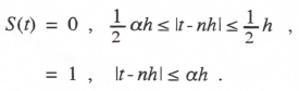
For a =1 the sampling process is continuous. As ![]() the sampling operation becomes instantaneous. For finite a we can expand the switch function in a Fourier series. Thus we let
the sampling operation becomes instantaneous. For finite a we can expand the switch function in a Fourier series. Thus we let
(5.66) 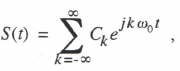
Where ![]() , the sample frequency in radians per second. The Fourier coefficients are given by the formula
, the sample frequency in radians per second. The Fourier coefficients are given by the formula
(5.67) 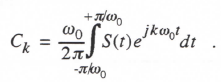
From Eq. (5.65) we have
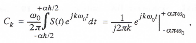
or
(5.68) 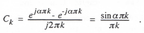
For ![]() , i.e.,
, i.e., ![]() becomes
becomes
(5.69) ![]()
Thus for a very short duty cycle a, the Fourier coefficients for the fundamental frequency ![]() and the lower harmonics (k = ± 2, ± 3, etc.,) are all equal approximately to a.
and the lower harmonics (k = ± 2, ± 3, etc.,) are all equal approximately to a.
Substituting Eq. (5.66) into Eq. (5.64), we obtain
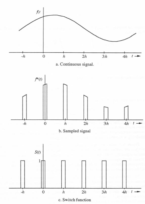
Figure 5.12 Sampling process
(5.70) 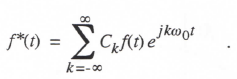
To obtain the frequency domain representation of f*(t) we take the Fourier transform of f*(t). Thus
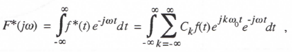
or
(5.71) 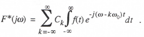
But the Fourier transform of f(t) is given by
(5.72) 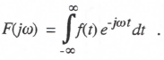
Thus we can write Eq. (5.70) as
(5.73) 
Eq. (5.73) shows that the spectrum ![]() of the sample function f*(t) is the sum of the original spectrum
of the sample function f*(t) is the sum of the original spectrum ![]() and the original spectrum shifted by
and the original spectrum shifted by ![]() . Furthermore, for near instantaneous sampling (a << 1), all the translated spectra will have essentially the same amplitude
. Furthermore, for near instantaneous sampling (a << 1), all the translated spectra will have essentially the same amplitude ![]() until k becomes quite large in magnitude.
until k becomes quite large in magnitude.
Figure 5.13 shows this result graphically, where for simplicity only the magnitudes ![]() and
and ![]() are plotted versus
are plotted versus ![]() . Note that for frequencies
. Note that for frequencies ![]() , the spectrum
, the spectrum ![]() of the continuous signal f(t) “folds back” on itself in the spectrum of
of the continuous signal f(t) “folds back” on itself in the spectrum of ![]() of the sample signal f*(t). This means that frequencies in f(t) that are larger than one-half the sample frequency
of the sample signal f*(t). This means that frequencies in f(t) that are larger than one-half the sample frequency ![]() , will show up as frequencies below one-half the sample frequency in f*(t). In fact, a frequency in f(t) equal to
, will show up as frequencies below one-half the sample frequency in f*(t). In fact, a frequency in f(t) equal to ![]() will be converted to zero frequency, i.e., a constant offset or bias in f*(t) .
will be converted to zero frequency, i.e., a constant offset or bias in f*(t) .
This foldback phenomena, called aliasing, can be prevented by passing f(t), the continuous signal, through a low-pass analog filter before sampling. This is an important consideration in interfacing a real-time digital simulation to analog inputs. If the analog signals have significant frequency content above one-half the sample frequency, which, for example, would be the case when the analog signals contain high-frequency noise, then the signals should be passed through a low-pass filter before being sampled for A to D conversion.
Determining the order and cutoff frequency for the low-pass filter involves a tradeoff. The lower the cutoff frequency ![]() , which must be below
, which must be below ![]() , the larger the accompanying phase lag. In addition, input components of f(t) with frequencies which are below
, the larger the accompanying phase lag. In addition, input components of f(t) with frequencies which are below ![]() but above
but above ![]() will be lost. Also, the higher the order n of the low-pass filter, the larger will be the accompanying phase lag for a given
will be lost. Also, the higher the order n of the low-pass filter, the larger will be the accompanying phase lag for a given ![]() . On the other hand, the larger the order n and the lower the cutoff frequency
. On the other hand, the larger the order n and the lower the cutoff frequency ![]() , the higher the attenuation of the unwanted frequencies in f(t) above
, the higher the attenuation of the unwanted frequencies in f(t) above ![]() .
.
Figure 5.13. Frequency spectrum, ![]() , of the continuous signal f(t), and frequency spectrum,
, of the continuous signal f(t), and frequency spectrum, ![]() , of the sample signal, f*(t).
, of the sample signal, f*(t).
Note that a sinusoidal data sequence ![]() can be viewed as a sample function r*(t) derived from a continuous signal
can be viewed as a sample function r*(t) derived from a continuous signal ![]() , where the duty cycle
, where the duty cycle ![]() . Then the single spectral frequency
. Then the single spectral frequency ![]() contained in f(t) will be transformed in r*(t) to the frequencies
contained in f(t) will be transformed in r*(t) to the frequencies ![]() , as shown in Figure 5.14. For those frequencies contained in r*(t), and hence
, as shown in Figure 5.14. For those frequencies contained in r*(t), and hence ![]() , which are greater than
, which are greater than ![]() , output DAC’s driven by
, output DAC’s driven by ![]() will respond in accordance with the DAC transfer function
will respond in accordance with the DAC transfer function ![]() or the combined compensator-DAC transfer function
or the combined compensator-DAC transfer function ![]() . In the DAC frequency response curves shown in Figures 5.5 and 5.8 the gain was plotted only up to
. In the DAC frequency response curves shown in Figures 5.5 and 5.8 the gain was plotted only up to ![]() , the sample frequency (equivalent to
, the sample frequency (equivalent to ![]() ). Figure 5.14 shows that the sinusoidal data sequence input to the DAC or compensated DAC will also contain frequencies above
). Figure 5.14 shows that the sinusoidal data sequence input to the DAC or compensated DAC will also contain frequencies above ![]() to which the DAC will respond. Reference to the various DAC and compensator-DAC gain formulas in Sections 5.3, 5.4 and 5.5 shows that in general the gain falls off with increasing frequency.
to which the DAC will respond. Reference to the various DAC and compensator-DAC gain formulas in Sections 5.3, 5.4 and 5.5 shows that in general the gain falls off with increasing frequency.
5.11. Multi-rate Input sampling and Averaging
In the previous section it was noted that frequencies above one-half the sample frequency ![]() of an A to D converter “fold-over” into frequencies below
of an A to D converter “fold-over” into frequencies below ![]() in the resulting digital data sequence. Since this is in general undesirable, each analog signal is normally passed through a low-pass analog filter with cutoff frequency below
in the resulting digital data sequence. Since this is in general undesirable, each analog signal is normally passed through a low-pass analog filter with cutoff frequency below ![]() . An alternative to passing f(t) through an
. An alternative to passing f(t) through an
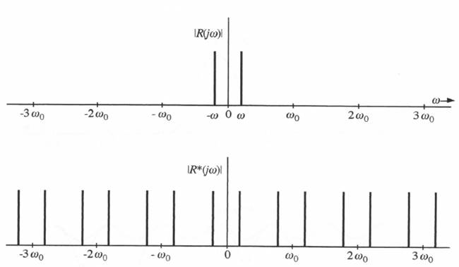
Figure 5.14. Spectrum ![]() of a continuous sinusoid of frequency
of a continuous sinusoid of frequency ![]() , and spectrum
, and spectrum ![]() of the sinusoid when sampled at frequency
of the sinusoid when sampled at frequency ![]() .
.
analog filter before sampling and A to D conversion is to perform the sampling and A to D conversion at a higher frame rate, one that is an integer multiple N of the original frame rate 1/h. The resulting fast data sequence is turned into a data sequence having the original frame rate by simply averaging every N successive samples to produce a single sample. The multi-rate sampling followed by averaging constitutes a low-pass digital filter. The single filter output for the nth frame is representative of the smoothed input halfway through the frame, i.e., ![]() . The effective time delay of this filter is h/2, where h is the period of the final output data sequence resulting from the A to D conversion process. This is because the algorithm which computes
. The effective time delay of this filter is h/2, where h is the period of the final output data sequence resulting from the A to D conversion process. This is because the algorithm which computes ![]() must wait until all N samples over the interval from t = nh to t = (n+1)h are received in order to compute the average, which then represents the smoothed data value at the midpoint of the nth frame. In this section we analyze the dynamics of the multi-rate sampling and averaging process in order to better understand how it can be used to improve the performance of simulations.
must wait until all N samples over the interval from t = nh to t = (n+1)h are received in order to compute the average, which then represents the smoothed data value at the midpoint of the nth frame. In this section we analyze the dynamics of the multi-rate sampling and averaging process in order to better understand how it can be used to improve the performance of simulations.
We first consider first the case where N = 2, with the samples of the continuous input f(t) taken at t = (n + 1/4)h and (n + 3/4)h. Note that the two samples are taken, respectively, at the midpoint of each of the two equal intervals into which the nth frame has been divided. Then the formula for ![]() is given by
is given by
(5.74) 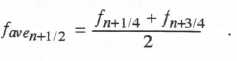
From the Z transform of Eq. (5.74) we obtain the following formula for the transfer function of the average for N = 2:

(5.75)
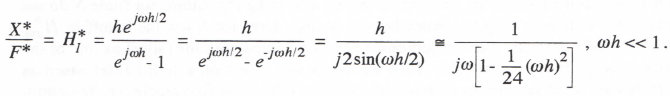
Note that there is no phase lag associated with ![]() , and that the gain error
, and that the gain error ![]() is approximately given by
is approximately given by ![]() for
for ![]() . Next consider the case where N = 3, with the samples given by
. Next consider the case where N = 3, with the samples given by ![]() and
and ![]() . Again, the samples are taken at the midpoint of each of the three equal intervals into which the nth frame is divided. The averager formula is then given by
. Again, the samples are taken at the midpoint of each of the three equal intervals into which the nth frame is divided. The averager formula is then given by
(5.76) 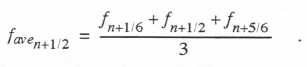
This results in the following transfer function for N = 3
(5.77) 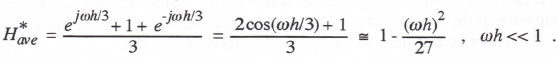
Again there is no phase lag, and here the gain error is approximately ![]() . For N = 4 the difference equation is given by
. For N = 4 the difference equation is given by
(5.78) 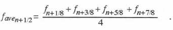
and the transfer function for N = 4 becomes
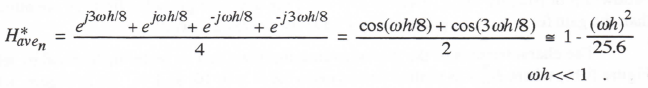
(5.79)
For the general case of N samples,
(5.80) 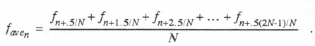
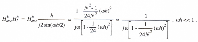
For this general case it can be shown that the approximate formula for the average transfer function, ![]() , is given by
, is given by
(5.81) 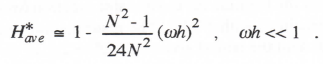
It is useful to examine the result when the number of samples N averaged over one frame approaches infinity. In this case the average of f(t) over the interval ![]() is given by the following formula:
is given by the following formula:
(5.82) 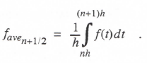
To derive the averager transfer function for sinusoidal inputs, we substitute ![]() into Eq. (5.82) and obtain
into Eq. (5.82) and obtain
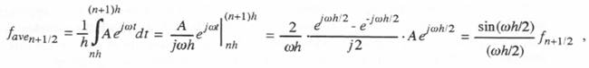
from which the averager transfer function for ![]() is given by
is given by
(5.83) 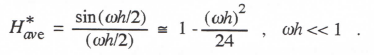
From Eq. (5.81) it is apparent that as the number N of multi-rate samples increases, the approximate gain error of the averager rapidly approaches the value given by ![]() for the case where
for the case where ![]() . Reference to Eqs. (5.75), (5.77) and (5.79) confirms this.
. Reference to Eqs. (5.75), (5.77) and (5.79) confirms this.
In Figure 5.15 is shown the exact transfer function, ![]() , versus dimensionless frequency
, versus dimensionless frequency ![]() , for
, for ![]() and
and ![]() . Also shown in the figure is the frequency response of a second-order analog low-pass filter with a damping ratio
. Also shown in the figure is the frequency response of a second-order analog low-pass filter with a damping ratio ![]() = 0.707 and a bandwidth of
= 0.707 and a bandwidth of ![]() , which is typical of the type which might be used to filter the inputs to A to D converters. Note the similarity of the digital transfer functions for different N over the frequency range
, which is typical of the type which might be used to filter the inputs to A to D converters. Note the similarity of the digital transfer functions for different N over the frequency range ![]() ; up to the basic frame sample frequency
; up to the basic frame sample frequency ![]() , i.e., the output sample frequency of the averaging algorithm, all of the averagers, regardless of N, behave approximately as low-pass filters with a bandwidth of roughly
, i.e., the output sample frequency of the averaging algorithm, all of the averagers, regardless of N, behave approximately as low-pass filters with a bandwidth of roughly ![]() . But for
. But for ![]() the averager gains for finite N are quite different than the gain for
the averager gains for finite N are quite different than the gain for ![]() , as given in Eq. (5.82) by
, as given in Eq. (5.82) by ![]() .
.
The characteristics of the digital averaging filters can be better understood by reference to Figure 5.16, where ![]() is plotted versus
is plotted versus ![]() for N = 9, 10, and
for N = 9, 10, and ![]() . As in Figure 5.15 we see that up to the sample frequency
. As in Figure 5.15 we see that up to the sample frequency ![]() the transfer functions are almost identical. But as
the transfer functions are almost identical. But as ![]() increases beyond
increases beyond ![]() ,
, ![]() for both N = 9 and 10 begins to diverge from
for both N = 9 and 10 begins to diverge from ![]() for
for ![]() . In particular, at
. In particular, at ![]() the transfer function for N = 9 is back up to unity. Although not shown in the figure,
the transfer function for N = 9 is back up to unity. Although not shown in the figure, ![]() for N = 9 will in fact repeat itself for increasing
for N = 9 will in fact repeat itself for increasing ![]() with a period of 9 on the dimensionless frequency scale,
with a period of 9 on the dimensionless frequency scale, ![]() . The reason for this becomes clear when we consider the averaging algorithm of Eq. (5.80) for N = 9. In order to take the Z transform of Eq. (5.80) we must rewrite the difference equation so that all the samples occur at integer step times. This requires using a step size of h/N = h/9. Then the formula for the transfer function for sinusoidal inputs is obtained from the Z transform by replacing
. The reason for this becomes clear when we consider the averaging algorithm of Eq. (5.80) for N = 9. In order to take the Z transform of Eq. (5.80) we must rewrite the difference equation so that all the samples occur at integer step times. This requires using a step size of h/N = h/9. Then the formula for the transfer function for sinusoidal inputs is obtained from the Z transform by replacing ![]() with
with ![]() . The resulting transfer function will then be periodic in the frequency domain, with the period given by
. The resulting transfer function will then be periodic in the frequency domain, with the period given by ![]() , or
, or ![]() .
.
On the other hand, when N = 10, reference to Eq. (5.80) shows that the step size for the algorithm must be given by h/2N = h/20 in order to have all the samples occur at integer step times. This is because the single output per frame h occurs halfway between two input samples when N is even. The resulting transfer function will have a frequency-domain periodicity of ![]() or
or ![]() for N = 10. In Figure 5.16 only the first half period of
for N = 10. In Figure 5.16 only the first half period of ![]() for N = 10 is visible.
for N = 10 is visible.
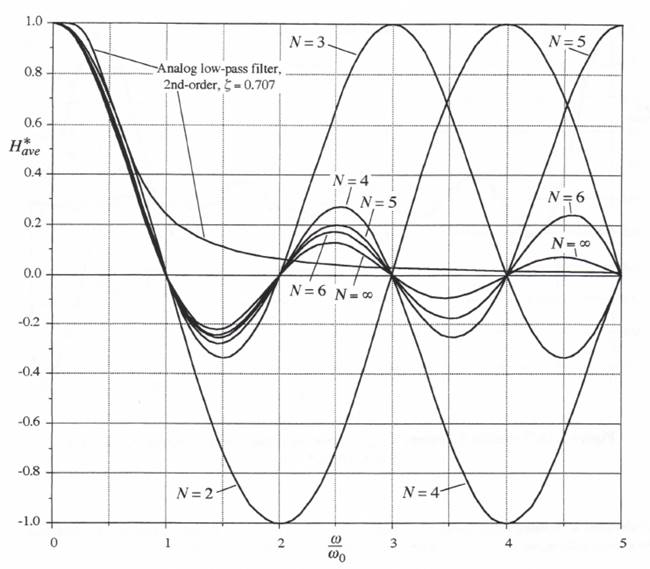
Figure 5.15. Transfer function, ![]() , for average of N samples per frame versus dimensionless frequency
, for average of N samples per frame versus dimensionless frequency ![]() , where
, where ![]() sample frequency of frame.
sample frequency of frame.
We therefore conclude that the gains of the digital averaging algorithms for finite N do not continue to fall off with increasing frequency beyond ![]() . Even for
. Even for ![]() the falloff in
the falloff in ![]() for
for ![]() is relatively gradual (gain proportional to 1/
is relatively gradual (gain proportional to 1/ ![]() ) compared with the falloff as
) compared with the falloff as ![]() of the second-order analog filter in Figure 5.15. Thus we cannot rely solely on a digital filter based on averaging multi-rate input samples to eliminate the aliasing effects for frequencies in the continuous input
of the second-order analog filter in Figure 5.15. Thus we cannot rely solely on a digital filter based on averaging multi-rate input samples to eliminate the aliasing effects for frequencies in the continuous input ![]() that are well beyond the basic frame sample frequency
that are well beyond the basic frame sample frequency ![]() . A low-pass analog filter prior to either single or multi-rate sampling is still the most effect means for accomplishing this.
. A low-pass analog filter prior to either single or multi-rate sampling is still the most effect means for accomplishing this.
What the multi-rate averaging filter does do, especially for large N, is reduce the effect of aliasing. It also provides an output ![]() which, when integrated numerically in the simulation of the system for which
which, when integrated numerically in the simulation of the system for which ![]() is the input, gives a much more accurate result than would otherwise
is the input, gives a much more accurate result than would otherwise
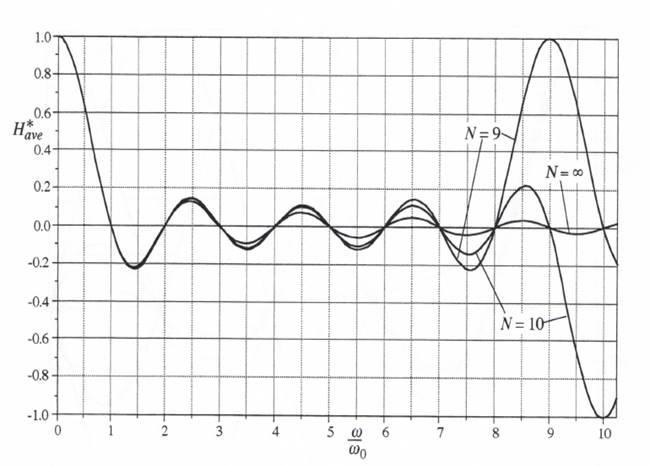
Figure 5.16. Transfer function, ![]() , versus dimensionless frequency
, versus dimensionless frequency ![]() for N = 9, 10 and
for N = 9, 10 and ![]() .
.
be obtained with integration formulas using ![]() or
or ![]() as inputs. To understand this we consider the simple state equation
as inputs. To understand this we consider the simple state equation ![]() when integrated by the following algorithm:
when integrated by the following algorithm:
(5.84) ![]()
Taking the Z transform using a step size of h/2, we obtain the following formula for the integrator transfer function:
(5.85)
Comparison of Eq. (5.85) with Eq. (3.37) shows that the integration algorithm given by Eq. (5.84) is of order ![]() with an integrator error coefficient
with an integrator error coefficient ![]() . If
. If ![]() in Eq. (5.84) is now replaced by
in Eq. (5.84) is now replaced by ![]() the transfer function of the resulting integration of the averaged samples of
the transfer function of the resulting integration of the averaged samples of ![]() to obtain the data sequence representing x will simply be the product
to obtain the data sequence representing x will simply be the product ![]() , which from Eqs. (5.81) and (5.85) is given by
, which from Eqs. (5.81) and (5.85) is given by
(5.86)
From Eq. (5.86) we see that ![]() is equal approximately to the ideal integrater transfer function,
is equal approximately to the ideal integrater transfer function, ![]() , with an additional gain error of
, with an additional gain error of ![]() . This error becomes very small indeed as the multi-rate input sampling ratio N becomes large. For
. This error becomes very small indeed as the multi-rate input sampling ratio N becomes large. For ![]() the error vanishes. This is also evident in Eq. (5.82), which shows that
the error vanishes. This is also evident in Eq. (5.82), which shows that ![]() for
for ![]() simply the area under f(t) over the integration frame. Thus when
simply the area under f(t) over the integration frame. Thus when ![]() for
for ![]() replaces
replaces ![]() in Eq. (5.84), the next state
in Eq. (5.84), the next state ![]() is simply the current state
is simply the current state ![]() plus the area under the f(t) versus t curve over the nth time frame.
plus the area under the f(t) versus t curve over the nth time frame.
For those components of f(t) with frequencies beyond ![]() , the state equation with f(t) as the input will indeed often behave approximately as a simple integrator. For example, this will typically be the case when f(t) represents an input acceleration to a mechanical dynamic system, in which case x represents the velocity state in the equation
, the state equation with f(t) as the input will indeed often behave approximately as a simple integrator. For example, this will typically be the case when f(t) represents an input acceleration to a mechanical dynamic system, in which case x represents the velocity state in the equation ![]() . Under these conditions the integration accuracy represented by Eq. (5.86) is actually realized when using multi-rate input sampling and averaging.
. Under these conditions the integration accuracy represented by Eq. (5.86) is actually realized when using multi-rate input sampling and averaging.