Dynamics of Real-Time Simulation – Chapter 6 – Special Methods for Simulating Linear Systems
6.1 Introduction In the simulation of dynamic systems it is often found that at least portions of the system can be described by linear ordinary differential equations. For example, control systems, although generally nonlinear, will frequently contain linear subsystems which are linear, such as controllers and/or linear filters. Also, elastic modes in flexible structures are often modelled using normal or generalized coordinates, which are represented by lightly damped second-order linear systems. In such cases it is usually more computationally efficient to employ specialized techniques for simulating these linear subsystems instead of standard integration algorithms. One of the techniques which has been widely used is the state-transition method. Another technique is Tustin’s substitution method, which is simply trapezoidal integration. In this chapter we describe these techniques and analyze their dynamic accuracy in the simulation of linear systems. We will employ the same error measures used in the previous chapters, namely, the characteristic root and sinusoidal transfer function errors in the form of asymptotic formulas for small dimensionless integration step sizes. 6.2 The State-transition Method The state-transition method is based on the analytic solution of the linear state equations over the integration step h in terms of the state-transition matrix*. By definition the method produces solutions that have characteristic roots which match exactly the roots of the linear system being simulated. This in turn means that the method permits any integration step size h without causing instability, if the system being simulated is itself stable. The state-transition method does, however, involve the evaluation of a definite integral which contains the input function and the state-transition matrix. The computer evaluation of this definite integral for arbitrary input functions represented as data sequences can only be approximate. This is where the state-transition method introduces dynamic errors into the simulation of linear systems. We will examine these dynamic errors in the frequency domain for various numerical methods of evaluating the definite integral. In particular, we will determine the transfer function gain and phase errors which each method produces as a function of the step size h, the input frequency w, and the zeros and poles of the linear system being simulated. These gain and phase errors will then be compared with those produced by both conventional integration algorithms and other specialized algorithms. The transfer function gain and phase error comparisons will show that in many cases the state-transition method is less accurate than conventional integration methods, e.g., when the input frequencies are well below the bandwidth of the linear system being simulated. We will also show that evaluation of the definite integral based on analytic approximations to the input function over the interval of integration can lead to transfer function gain and phase errors which are completely independent of the system being simulated and depend only on coh, the product of the frequency and the step size. * See, for example, Chen, C.T., Introduction to Linear System Theory, Holt, Reinhart and Winston, Inc., 1960. We will assume that the linear system being simulated is of order k and has m scalar inputs. The system can be represented by the following state vector equation: (6.1)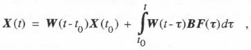 where W(t) is the kxk state-transition matrix. Thus the element
 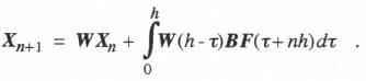 For F = 0 and any initial condition X(0) = X0, the difference equation represented by Eq. (6.3) produces a digital solution X1, X2, X3, … which will be exactly correct at the discrete times h, 2h, 3h, … , respectively. This means that the characteristic roots of the digital solution will also be exact. Any dynamic errors exhibited by the state-transition method will result from the numerical method chosen to calculate the definite integral in Eq. (6.3).
To illustrate the use of the state-transition method we consider the first-order linear system represented by the equation
(6.4)
For F = 0 and any initial condition X(0) = X0, the difference equation represented by Eq. (6.3) produces a digital solution X1, X2, X3, … which will be exactly correct at the discrete times h, 2h, 3h, … , respectively. This means that the characteristic roots of the digital solution will also be exact. Any dynamic errors exhibited by the state-transition method will result from the numerical method chosen to calculate the definite integral in Eq. (6.3).
To illustrate the use of the state-transition method we consider the first-order linear system represented by the equation
(6.4) 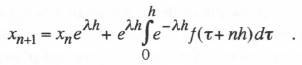 The simplest way to evaluate the definite integral is to use rectangular integration. Thus we let the integrand be equal to its value at t = 0, in which case the integral becomes simply hf(nh) = hfn, and Eq. (6.6) becomes
* Chen, op. cit.
(6.7)
The simplest way to evaluate the definite integral is to use rectangular integration. Thus we let the integrand be equal to its value at t = 0, in which case the integral becomes simply hf(nh) = hfn, and Eq. (6.6) becomes
* Chen, op. cit.
(6.7) 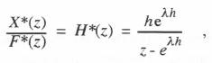 Where
Where 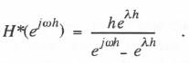 From Eq. (6.4) we see that the transfer function of the continuous system is
(6.10)
From Eq. (6.4) we see that the transfer function of the continuous system is
(6.10) 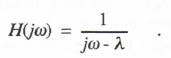 The fractional error in digital transfer function,
 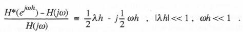 For any simulation of reasonable accuracy the complex number represented by the right side of Eq. (6.11) will have a magnitude which is small compared with unity. Earlier, in Eqs. (1.53) and (1.54) in Chapter 1, we showed that the real part of this complex number, denoted by
 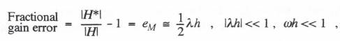 (6.13)
 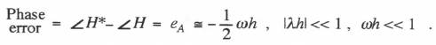 Note that the gain and phase errors both vary as the first power of the step size h. This is to be expected, since we used rectangular integration to approximate the definite integral in Eq. (6.6). Note also the the phase error corresponds to a time delay of h/2, which again is representative of rectangular integration.
An alternative method of evaluating the definite integral in Eq. (6.6) is to approximate the input over the interval h by a constant
Note that the gain and phase errors both vary as the first power of the step size h. This is to be expected, since we used rectangular integration to approximate the definite integral in Eq. (6.6). Note also the the phase error corresponds to a time delay of h/2, which again is representative of rectangular integration.
An alternative method of evaluating the definite integral in Eq. (6.6) is to approximate the input over the interval h by a constant 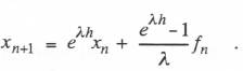 This results in the following system Z transform:
(6.15)
This results in the following system Z transform:
(6.15) 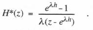 With the same method used to obtain Eqs. (6.12) and (6.13) from (6.8), we obtain the following approximate formulas for the transfer function gain and phase errors in this case:
(6.16)
With the same method used to obtain Eqs. (6.12) and (6.13) from (6.8), we obtain the following approximate formulas for the transfer function gain and phase errors in this case:
(6.16) 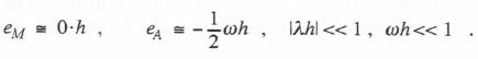 Here the gain
 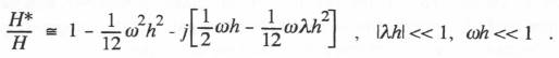 The formulas for
  We note that the gain error of order
 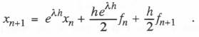 Based on this difference equation we obtain the following asymptotic formulas for the transfer function gain and phase errors:
(6.20)
Based on this difference equation we obtain the following asymptotic formulas for the transfer function gain and phase errors:
(6.20) 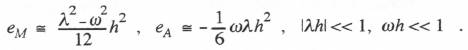 Note that the gain and phase errors are proportional to
 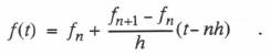 When the integral in Eq. (6.6) is evaluated in this case, the following difference equation is obtained:
(6.22)
When the integral in Eq. (6.6) is evaluated in this case, the following difference equation is obtained:
(6.22) 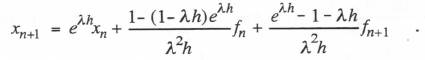 From this difference equation we obtain the following approximate formulas for the transfer function gain and phase errors:
(6.23)
From this difference equation we obtain the following approximate formulas for the transfer function gain and phase errors:
(6.23) 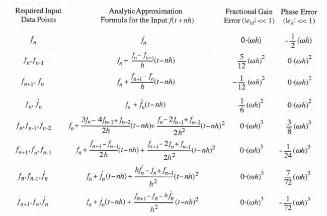 Comparison of the formulas in Table 6.1 for the transfer function errors with the individual integrator transfer function errors which are summarized in Table 3.1 of Section 3.12 shows that the formulas are identical for the same f(t) approximation forms. For example, Table 3.1 shows that the AB-2 integrator transfer function is given by the following approximate formula:
(6.24)
Comparison of the formulas in Table 6.1 for the transfer function errors with the individual integrator transfer function errors which are summarized in Table 3.1 of Section 3.12 shows that the formulas are identical for the same f(t) approximation forms. For example, Table 3.1 shows that the AB-2 integrator transfer function is given by the following approximate formula:
(6.24) 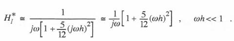 Thus the AB-2 integrator has a gain error equal to
 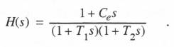 Eq. (6.25) represents a typical bandwidth-limited proportional plus rate controller which would be used in a feedback control system. First we represent the system as the sum of two first-order systems. Thus we let
(6.26)
Eq. (6.25) represents a typical bandwidth-limited proportional plus rate controller which would be used in a feedback control system. First we represent the system as the sum of two first-order systems. Thus we let
(6.26) 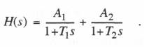 Using Eq. (1.44), we obtain the following formulas for the constants
 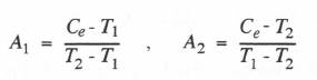 Each of the first-order systems in Eq. (6.26) can be simulated by utilizing any of the state-transition formulations described in the previous section. The method which represents the input f(t) as a linear time function based on
  Noting that
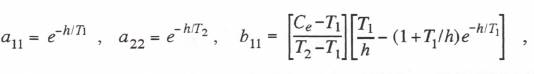
 (6.29)
From Eq. (6.26) it follows that the controller output X is simply the sum of the two state variables X 1 and X 2. Thus
(6.30)
(6.29)
From Eq. (6.26) it follows that the controller output X is simply the sum of the two state variables X 1 and X 2. Thus
(6.30)  Comparison with H(s) in Eq. (6.25) shows that
(6.32)
Comparison with H(s) in Eq. (6.25) shows that
(6.32)  Thus the general transient solution for X 1 and X 2 becomes
(6.37)
Thus the general transient solution for X 1 and X 2 becomes
(6.37) 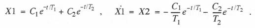 First we obtain the solution for X 1(0) = 1, X 2(0) = 0. With these initial conditions, Eq. (6.37) gives us
 from which C1 = T1/(T1 –T2) and C2 = T2/(T2 –T1). Thus Eq. (6.37) becomes
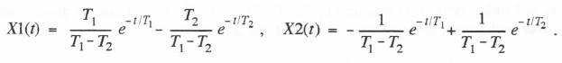 (6.38)
To obtain the solution for X 1(0) = 0, X 2(0) = 1, we follow the same procedure, which results in
the following solutions:
(6.38)
To obtain the solution for X 1(0) = 0, X 2(0) = 1, we follow the same procedure, which results in
the following solutions:
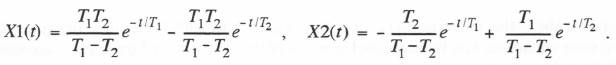 (6.39)
In Eq. (6.38), X 1(h) represents the response at t = h to a unit initial condition on X 1. Thus X 1(h) = w 1 1 for the state-transition matrix W in the vector differential equation given by (6.3). Similarly, in Eq. (6.38) X 2(h) = w21, the solution for X2 at t = h for a unit initial condition on X 1. In the same way, in Eq. (6.39) X 1(h) = w21 and X2(h) = w22. Thus the following formulas are obtained from Eqs. (6.38) and (6.39) for the elements of the 2×2 state-transition matrix of the linear system described by Eq. (6.33):
(6.39)
In Eq. (6.38), X 1(h) represents the response at t = h to a unit initial condition on X 1. Thus X 1(h) = w 1 1 for the state-transition matrix W in the vector differential equation given by (6.3). Similarly, in Eq. (6.38) X 2(h) = w21, the solution for X2 at t = h for a unit initial condition on X 1. In the same way, in Eq. (6.39) X 1(h) = w21 and X2(h) = w22. Thus the following formulas are obtained from Eqs. (6.38) and (6.39) for the elements of the 2×2 state-transition matrix of the linear system described by Eq. (6.33):
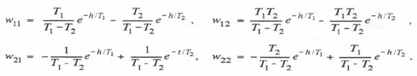 (6.40)
We now turn to the calculation of the definite integral in Eq. (6.3), where we will use the same analytic approximation to the input f(t) that was employed earlier in this section. Thus we represent f(t) with the linear formula in Eq. (6.21). This, along with the formulas in Eq. (6.40) for the state-transition matrix elements, permits us to determine analytically the definite integral in Eq. (6.3). Alternatively, based on Eq. (6.21), we see that the definite integral represents the response to a step input of amplitude
(6.40)
We now turn to the calculation of the definite integral in Eq. (6.3), where we will use the same analytic approximation to the input f(t) that was employed earlier in this section. Thus we represent f(t) with the linear formula in Eq. (6.21). This, along with the formulas in Eq. (6.40) for the state-transition matrix elements, permits us to determine analytically the definite integral in Eq. (6.3). Alternatively, based on Eq. (6.21), we see that the definite integral represents the response to a step input of amplitude 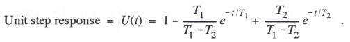 Since a unit ramp function is the time integral of a unit step function, the unit ramp response, V(t), will be the time integral of the unit step response, U(t). Integrating Eq. (6.41) and choosing the integration constant such that V(0) = 0, we obtain
(6.42)
Since a unit ramp function is the time integral of a unit step function, the unit ramp response, V(t), will be the time integral of the unit step response, U(t). Integrating Eq. (6.41) and choosing the integration constant such that V(0) = 0, we obtain
(6.42) 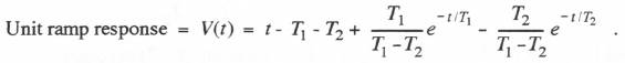 For the second-order system represented by Eq. (6.33), with Eq. (6.21) used to approximate the input f(t) over each frame, the state-transition equations take the form
(6.43)
For the second-order system represented by Eq. (6.33), with Eq. (6.21) used to approximate the input f(t) over each frame, the state-transition equations take the form
(6.43) 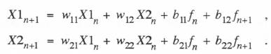 We have noted above that the term
 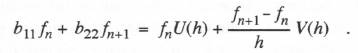 Since X 2 =
 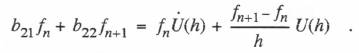 Here we have replaced
 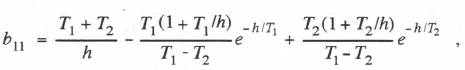 (6.47)
 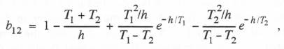 (6.48)
 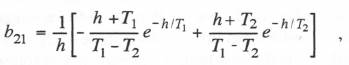 (6.49)
 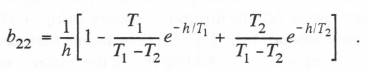 From Eq. (6.34) we see that the formula used to compute the final controller output X at the n+ 1 frame is given by
(6.50)
From Eq. (6.34) we see that the formula used to compute the final controller output X at the n+ 1 frame is given by
(6.50) 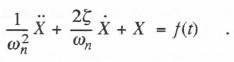 The characteristic roots for
 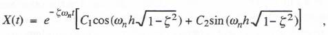 where C1 and C2 are constants. We let the state variables X1 and X2 be defined as X1 = X and X2 = X in Eq. (6.51). As in the previous section, we first determine C1 and C2 for the initial conditions X1(0) =1, X2(0) = 0. The resulting solutions for X1(h) and X2(h) correspond to w11 and w21, respectively. In the same way, for initial conditions X1( 0) = 0, X2(0) = 1, the solutions for X1( h) and X2(h) correspond to w12 and w22 , respectively. In this manner we obtain the following formulas for the elements of the 2×2 state-transition method when
 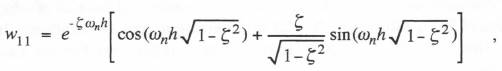 (6.55)
 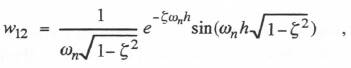 (6.56)
 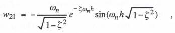 (6.57)
 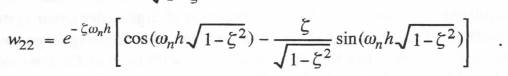 Next we determine the unit step and unit ramp response functions in order to be able to construct the definite integral formulas when first-order analytic approximations to the input f(t) are utilized in the state-transition method. Consider first the unit step response, U(t). For f(t) = 1 in Eq. (6.51), it is evident that the steady-state response X(t) = 1. Adding this to the transient solution of Eq. (6.53) and solving for the constants C1 and C2 with zero initial conditions, we obtain the following equation for the unit step response of the second-order system for
 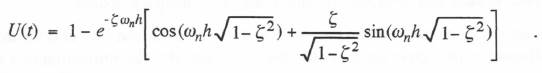 The unit ramp response will simply be the time integral of the unit step response. Alternatively, for a unit ramp input, f(t) = t, it is easy to show by substitution into Eq. (6.51) that
 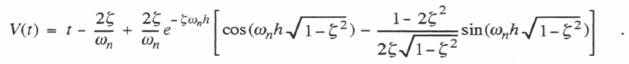 (6.59)
If we use the first-order analytic approximation to the input f(t) based on
(6.59)
If we use the first-order analytic approximation to the input f(t) based on 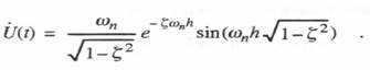 From Eqs. (6.58) through (6.61) we can now determine the formulas for calculating the coefficients b11, b12, b21 and b22 for the underdamped second-order system considered in this section. Eqs. (6.54) through (6.57) give the formulas for the coefficients w11, w12, w21 and w22.
If our first-order linear approximation to f(t) is based on
From Eqs. (6.58) through (6.61) we can now determine the formulas for calculating the coefficients b11, b12, b21 and b22 for the underdamped second-order system considered in this section. Eqs. (6.54) through (6.57) give the formulas for the coefficients w11, w12, w21 and w22.
If our first-order linear approximation to f(t) is based on 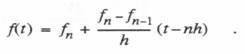 In this case the state-transition difference equation takes the form
(6.63)
In this case the state-transition difference equation takes the form
(6.63) 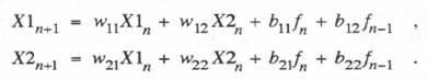 From Eq. (6.62) it is easily seen that the formulas for the coefficients b11, b12, b21 and b22, in terms of the unit step and unit ramp response functions, in this case become
 In terms of unit step and ramp response functions, the coefficients b11, b12, b21 and b22 become
(6.67)
In terms of unit step and ramp response functions, the coefficients b11, b12, b21 and b22 become
(6.67) 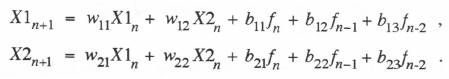 Based on the formula in Table 6.1 for the quadratic approximation to f(t) that utilizes
  (6.69)
In the second equation of (6.69) we have replaced
(6.69)
In the second equation of (6.69) we have replaced 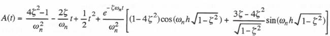 (6.70)
The above equation for A(t), along with U(t) in Eq. (6.58), V(t) in Eq. (6.59), and U(t) in Eq.(6.61), can be used in formulas similar to those in Eq. (6.69) to compute the appropriate coefficients for any of the other three quadratic f(t) approximations listed in Table 6.1.
To obtain A(t) for the overdamped second-order system of the previous section we note from Eq. (6.33) that the steady-state response for a unit acceleration input is given by
(6.70)
The above equation for A(t), along with U(t) in Eq. (6.58), V(t) in Eq. (6.59), and U(t) in Eq.(6.61), can be used in formulas similar to those in Eq. (6.69) to compute the appropriate coefficients for any of the other three quadratic f(t) approximations listed in Table 6.1.
To obtain A(t) for the overdamped second-order system of the previous section we note from Eq. (6.33) that the steady-state response for a unit acceleration input is given by 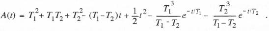 This equation for A(t), along with U(t) in Eq. (6.41) and V(t) in Eq. (6.43), can now be used to determine state-transition difference equation coefficients when using any of the quadratic formulas in Table 6.1 as an analytic approximation for f(t).
6.6 The State-transition Method in the Case of Repeated Roots
In this section we consider a second-order system with repeated roots, i.e., one where both characteristic roots are the same. This corresponds to
This equation for A(t), along with U(t) in Eq. (6.41) and V(t) in Eq. (6.43), can now be used to determine state-transition difference equation coefficients when using any of the quadratic formulas in Table 6.1 as an analytic approximation for f(t).
6.6 The State-transition Method in the Case of Repeated Roots
In this section we consider a second-order system with repeated roots, i.e., one where both characteristic roots are the same. This corresponds to 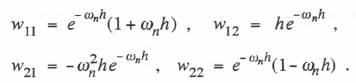 The above formulas can also be obtained by letting
 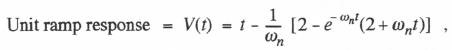 (6.77)
 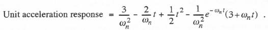 With the formulas in Eqs. (6.73) through (6.77) we can determine the coefficients in the state-transition difference equations using analytic approximations up to second-order for the input f(t). The procedure to do this for the repeated-root system considered in this section is the same as that presented in the previous section for the underdamped second-order system.
In Section 6.4 we considered the simulation of a linear controller. The second-order controller transfer function in Eq. (6.25) was represented in Eq. (6.26) as the sum of two first-order transfer functions. The state-transition method was then used to simulate each first-order system. However, when the two controller time constants, T1 and T2, are equal, the second-order transfer function can no longer be represented as the sum of two first-order transfer functions. This is apparent in the formulas of Eq. (6.27). In this case the controller must be simulated directly as a second-order system. When T1 = T2, both characteristic roots are the same, and the formulas developed in this section for repeated roots when using the state-transition method can be used. Note also that if the two characteristic roots of the controller are complex, the controller must also be simulated directly as a second-order system. In this case the state-transition formulation developed in Section 6.5 applies.
After introducing and analyzing Tustin’s method in the next section, we will make some specific transfer function accuracy comparisons with the state-transition method. This will enable us to better understand some of the relative advantages and disadvantages of these two schemes in simulating linear systems.
6.7 Tustin’s Method
We now turn to the consideration of Tustin’s substitution method for the simulation of linear systems.* Actually, the method is simply trapezoidal integration, which we have already analyzed in Section 3.5 of Chapter 3 as one of the single-pass implicit integration algorithms. From Eq. (3.81) we have the following formula for the Z transform of the trapezoidal integrator:
(6.78)
With the formulas in Eqs. (6.73) through (6.77) we can determine the coefficients in the state-transition difference equations using analytic approximations up to second-order for the input f(t). The procedure to do this for the repeated-root system considered in this section is the same as that presented in the previous section for the underdamped second-order system.
In Section 6.4 we considered the simulation of a linear controller. The second-order controller transfer function in Eq. (6.25) was represented in Eq. (6.26) as the sum of two first-order transfer functions. The state-transition method was then used to simulate each first-order system. However, when the two controller time constants, T1 and T2, are equal, the second-order transfer function can no longer be represented as the sum of two first-order transfer functions. This is apparent in the formulas of Eq. (6.27). In this case the controller must be simulated directly as a second-order system. When T1 = T2, both characteristic roots are the same, and the formulas developed in this section for repeated roots when using the state-transition method can be used. Note also that if the two characteristic roots of the controller are complex, the controller must also be simulated directly as a second-order system. In this case the state-transition formulation developed in Section 6.5 applies.
After introducing and analyzing Tustin’s method in the next section, we will make some specific transfer function accuracy comparisons with the state-transition method. This will enable us to better understand some of the relative advantages and disadvantages of these two schemes in simulating linear systems.
6.7 Tustin’s Method
We now turn to the consideration of Tustin’s substitution method for the simulation of linear systems.* Actually, the method is simply trapezoidal integration, which we have already analyzed in Section 3.5 of Chapter 3 as one of the single-pass implicit integration algorithms. From Eq. (3.81) we have the following formula for the Z transform of the trapezoidal integrator:
(6.78) 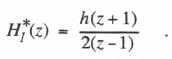 As noted in Section 3.3,
 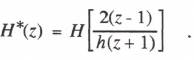 When we apply this formula to the controller transfer function given in Eq. (6.25), we obtain the
* See Smith, Jon M., Mathematical Modeling & Digital Simulation for Engineers, John Wiley & Sons, 1077.
6-16
following Z transform:
When we apply this formula to the controller transfer function given in Eq. (6.25), we obtain the
* See Smith, Jon M., Mathematical Modeling & Digital Simulation for Engineers, John Wiley & Sons, 1077.
6-16
following Z transform:
 (6.81)
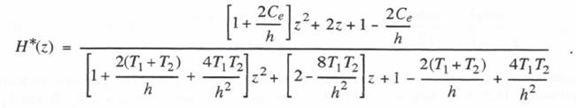
Based on Eq. (6.81) the difference equation for the controller output
(6.81)
Based on Eq. (6.81) the difference equation for the controller output 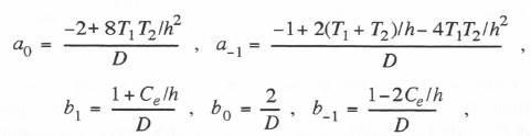 where
(6.84)
where
(6.84) 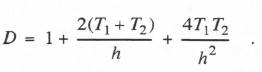 The difference equation in (6.82) requires 5 multiplications and 4 additions per integration step. When we simulate the controller as the sum of two first-order systems using the state-transition method, Eqs. (6.28) and (6.30) require 6 multiplications and 5 additions. When the controller is simulated as a single second-order system using the state-transition method, Eqs. (6.43) and (6.50) require 9 multiplications and 7 additions. With either mechanization it is clear that the state-transition method will require more processing time than Tustin’s method in simulating the controller.
Next we compare the dynamic accuracy of the two methods. For Tustin’s method (i.e., trapezoidal or second-order implicit integration) we see from Table 3.1 that the integrator error coefficient,
The difference equation in (6.82) requires 5 multiplications and 4 additions per integration step. When we simulate the controller as the sum of two first-order systems using the state-transition method, Eqs. (6.28) and (6.30) require 6 multiplications and 5 additions. When the controller is simulated as a single second-order system using the state-transition method, Eqs. (6.43) and (6.50) require 9 multiplications and 7 additions. With either mechanization it is clear that the state-transition method will require more processing time than Tustin’s method in simulating the controller.
Next we compare the dynamic accuracy of the two methods. For Tustin’s method (i.e., trapezoidal or second-order implicit integration) we see from Table 3.1 that the integrator error coefficient, 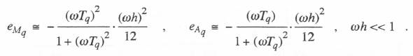 To obtain the gain and phase errors for the simulation of the overall controller transfer function represented by Eq. (6.25), we utilize Eqs. (3.69), (3.70) and (6.85) with Tq equal to T1, T2, and Ce for q = 1, 2 and 3, respectively. This results in the following formulas:
(6.86)
To obtain the gain and phase errors for the simulation of the overall controller transfer function represented by Eq. (6.25), we utilize Eqs. (3.69), (3.70) and (6.85) with Tq equal to T1, T2, and Ce for q = 1, 2 and 3, respectively. This results in the following formulas:
(6.86) 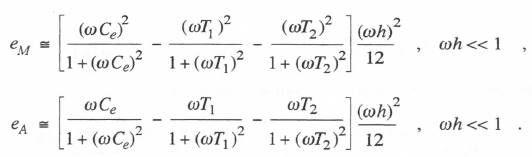 In order to compare the above gain and phase errors for Tustin’s method with those for the state-transition method, we consider a specific case. Let T1 = T2 = 0.1Ce. For these parameters the transfer function
 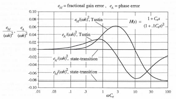 Figure 6.1. Normalized gain and phase errors versus
  (6.91)
and
(6.92)
(6.91)
and
(6.92)  where
where 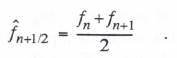 If we replace
 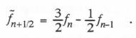 This is in fact the extrapolation formula in Table 4.1 with inputs
 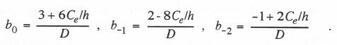 where D is given by the previous formula in Eq. (6.84).
On the other hand, if Eqs. (6.88), (6.90) and (6.92) are used for the trapezoidal-integration simulation of our bandwidth-limited controller, the correct difference equations for the case of real-time inputs can be obtained by simply replacing
where D is given by the previous formula in Eq. (6.84).
On the other hand, if Eqs. (6.88), (6.90) and (6.92) are used for the trapezoidal-integration simulation of our bandwidth-limited controller, the correct difference equations for the case of real-time inputs can be obtained by simply replacing 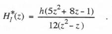 Substituting the reciprocal of
 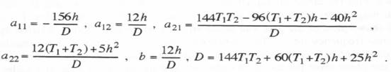 The implementation of third-order implicit integration using Eqs. (6.101), (6.102) and (6.103) requires 11 additions and 11 multiplications versus the 8 additions and 9 multiplications needed to implement the single difference equation given by Eq. (6.100). On the other hand, Eqs. (6.101), (6.102) and (6.103) pose a less severe startup problem.
If we use the state-transition method with the analytic approximation for the input f(t) based on
The implementation of third-order implicit integration using Eqs. (6.101), (6.102) and (6.103) requires 11 additions and 11 multiplications versus the 8 additions and 9 multiplications needed to implement the single difference equation given by Eq. (6.100). On the other hand, Eqs. (6.101), (6.102) and (6.103) pose a less severe startup problem.
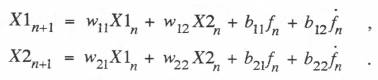
If we use the state-transition method with the analytic approximation for the input f(t) based on 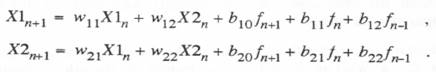 where the final output
 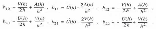 From Eqs. (6.105) and (6.103) we see that the state-transition method requires 11 multiplications and 9 additions per integration step. For the input representation based on
 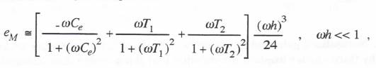 (6.107)
 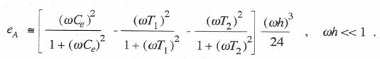 Comparison with the errors in Eq. (6.86) for Tustin’s method shows that the normalized error coefficient magnitudes for gain and phase here have simply reversed roles. For
 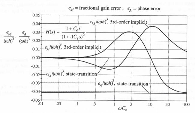 Figure 6.2. Normalized gain and phase errors versus
 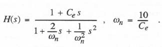 The state equations for the system can be written as
(6.110)
The state equations for the system can be written as
(6.110) 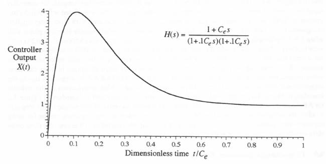 Figure 6.3. Unit-step response of controller.
We consider first the controller simulation using the state-transition method with the continuous input f(t) over the nth frame represented by a linear approximation based on
Figure 6.3. Unit-step response of controller.
We consider first the controller simulation using the state-transition method with the continuous input f(t) over the nth frame represented by a linear approximation based on 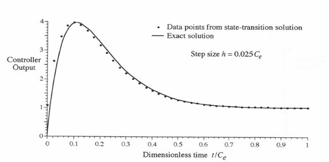 Figure 6.4. Unit step response of controller when simulated by the state-transition method based on
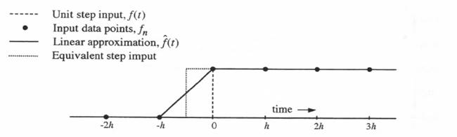 Figure 6.5. Linear interpolation function
 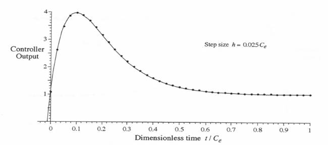 Figure 6.6. Comparison of state-transition method based on
 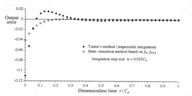 Figure 6.7. Controller simulation; comparison of unit step-response errors using Tustin’s method with errors using the state-transition method based on
 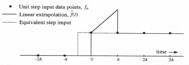 Figure 6.8. Linear extrapolation function
 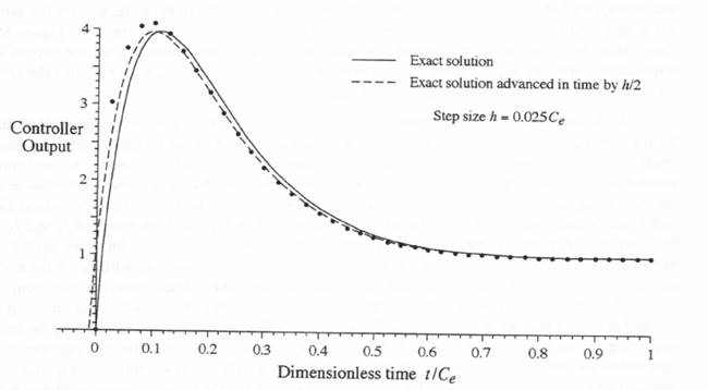 Figure 6.9. Unit step response of controller when simulated by the state-transition method based on
 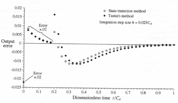 Figure 6.10. Controller simulation; comparison of unit step-response errors with both the state- transition and Tustin’s method based on inputs
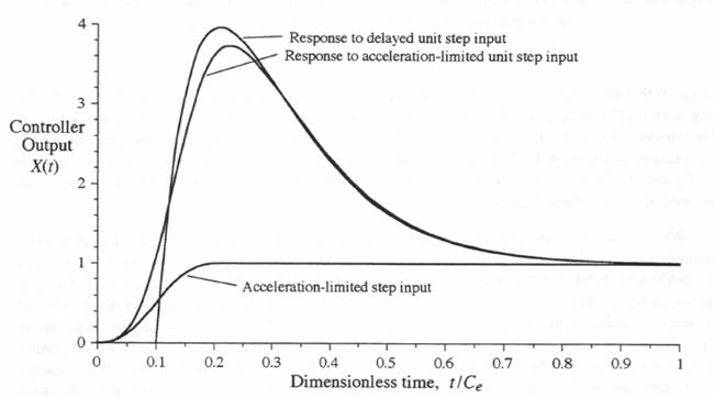 Figure 6.11. Controller response to an acceleration-limited step input.
For the same acceleration-limited step input, Figure 6.12 shows the output response error when the controller is simulated by Tustin’s method and by the state-transition method, where both methods use the input data points
Figure 6.11. Controller response to an acceleration-limited step input.
For the same acceleration-limited step input, Figure 6.12 shows the output response error when the controller is simulated by Tustin’s method and by the state-transition method, where both methods use the input data points 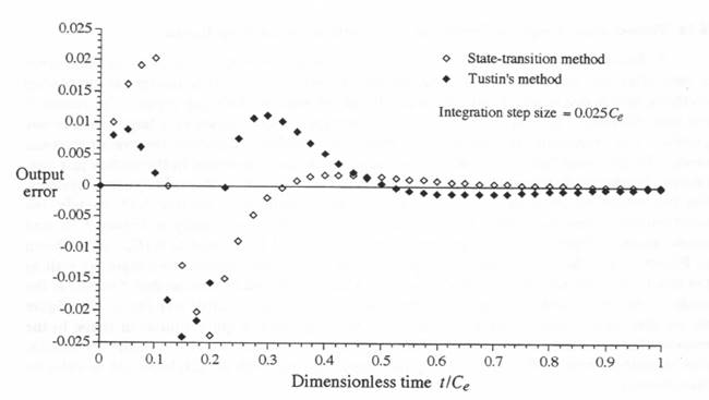 Figure 6.12. Output error in simulated controller response for an acceleration-limited step input based on input data points
 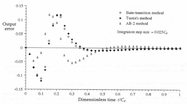 Figure 6.13. Output error in simulated controller response for an acceleration-limited step input based on input data points
 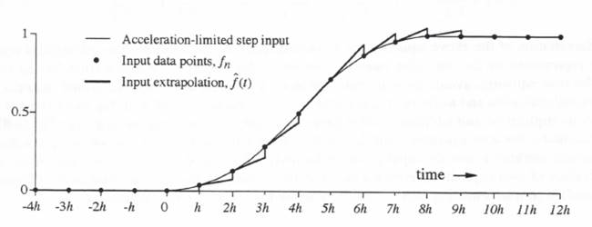 Figure 6.14. Linear extrapolation function
 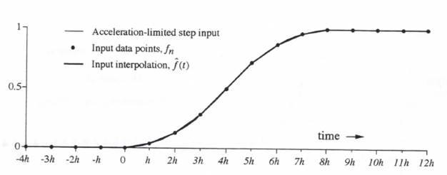 Figure 6.14. Linear interpolation function
 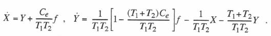 Differentiation of the above equation for